Greedy Algorithms The Greedy strategy is (just like D&C or DP) a - - PowerPoint PPT Presentation

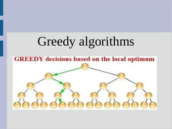
Greedy Algorithms

The Greedy strategy is (just like D&C or DP) a design paradigm. General idea: Greedy algorithms always make choices that “look best at the moment.” They do not always yield optimal results, but in many cases they do (and if not, then often “pretty close” to optimal).

Greedy Strategy 1

Huffman codes

Used for compressing data (savings 20% to 90%). Data is considered to be a sequence of characters. Huffman’s greedy algorithm

• computes frequency of occurrence of characters, and
• assigns binary strings to characters: the more frequent a character,

the shorter the string Results in binary character code (“code”).

Greedy Strategy 2

Consider file of length 100, 000, containing only characters a,b,c,d,e,f, and the following frequencies (in thousands). a b c d e f 45 13 12 16 9 5 With fixed length codes, exact code of each character does not matter (w.r.t. length). For six characters, we need three bits per character, a total of 300, 000 bits. With variable length codes, assignment does matter. Consider fol- lowing code. a b c d e f 101 100 111 1101 1100 Resulting length (in bits) now is (45 · 1 + 13 · 3 + 12 · 3 + 16 · 3 + 9 · 4 + 5 · 4) · 1, 000 = 224, 000

Greedy Strategy 3

Prefix codes

No codeword is prefix of some other codeword! Encoding is simple: just concatenate codewords. Using a b c d e f 101 100 111 1101 1100 the code for “deaf” is 111110101100. Prefix codes simplify decoding, they parse uniquely.

Greedy Strategy 4

Binary Tree Representation

We need convenient representation for prefix codes. Use binary tree:

• leaves represent characters,
• interpret binary codeword for a character as path from root to

corresponding leaf; 0 means “left”, 1 means “right”.

Greedy Strategy 5

Example: fixed length code character a b c d e f frequency 45 13 12 16 9 5 codeword 000 001 010 011 100 101

100 86 14 58 28 14 a:45 b:13 c:12 d:16 e:9 f:5 1 1 1 1 1

Leaves are labeled with character and frequency, interior vertices with sum of frequencies of leaves in sub-tree.

Greedy Strategy 6

Example: variable length code character a b c d e f frequency 45 13 12 16 9 5 codeword 101 100 111 1101 1100

30

c:12 d:16 b:13 e:9 f:5 a:45 1 1 1 1 1 30

100 55 25 14

Greedy Strategy 7

Optimal Codes

Optimal codesare always represented by a full binary tree, where every non-leaf vertex has two children (exercise).

• Fixed-length example therefore non-optimal (obviously, we already

have seen better one).

• Full binary trees =

⇒ if C is our alphabet, then |C| leaves and |C| − 1 internal vertices (exercise).

Greedy Strategy 8

Cost Model

Given tree T corresponding to a prefix code, we can compute number

• f bits to encode a file.

For c ∈ C, f(c) denotes frequency, and dT(c) denotes depth of c’s leaf. Then, cost of T is B(T) =

• c∈C

f(c) · dT(c) Note: dT(c) is also length of c’s codeword!

Greedy Strategy 9

Excursion: Min-priority queues

Huffman’s algorithm uses a min-priority queue (a heap with certain properties). Relevant operations: Build-Min-Heap: constructs the heap; takes O(n) for n items. Extract-Min: finds the minimal item and removes it from heap; takes O(log n) per operation. New: Insert: inserts new items into queue; takes O(log n). Increase-key: inserts new items into queue; takes O(log n).

Greedy Strategy 10

Excursion: Min-priority queues

Increase-key: It increases the key of the element (pointer as param- eter) and it compares the element with parent until heap-property is restored. Insert: Insert new element as a leaf and use Increase-key.

Greedy Strategy 11

Idea of the Algorithm

The idea of Huffman’s algorithm is as follows.

• Tree is built bottom-up.
• Begin with |C| leaves, then do |C| − 1 merging operations to

create final tree.

• In each merger,

– extract two least-frequent objects to merge; Result: new object whose frequency is sum of frequencies of two merged objects.

Greedy Strategy 12

Huffman’s greedy algorithm

1: n ← |C| 2: Q ← C

{Build-Min-Heap}

3: for i ← 1 to n − 1 do 4:

allocate new object z

5:

left[z] ← x ← Extract-Min(Q)

6:

right[z] ← y ← Extract-Min(Q)

7:

f[z] ← f[x] + f[y]

8:

Insert(Q, z)

9: end for

Running time Initialization takes O(n) and each heap operation in loop takes O(log n). Total running time is therefore O(n log n).

Greedy Strategy 13

Example

f:5 e:9 c:12 b:13 d:16 a:45 c:12 b:13 d:16 a:45 f:5 e:9 d:16 a:45 f:5 e:9 c:12 b:13 a:45 f:5 e:9 d:16 c:12 b:13 25 14 30 f:5 e:9 d:16 14 30 c:12 b:13 25 a:45 55 f:5 e:9 d:16 14 30 c:12 b:13 25 a:45 14 14 25 55 100 1 1 1 1 1 1 1 1 1 1 1 1 1 1 1

Greedy Strategy 14

Correctness

Definition: Let C be alphabet, character c ∈ C has frequency f[c]. Lemma 1. Let x and y two characters in C with lowest frequency. Then there is optimal prefix code for C in which codewords for x and y have same length and differ in only one bit. In words: building up tree can w.l.o.g. begin with greedy choice of merging lowest-frequency characters.

Greedy Strategy 15

Proof.

• Let T be any optimal tree.
• Let a and b characters that are sibling leaves of maximum depth

in T.

• W.l.o.g. f[a] ≤ f[b] and f[x] ≤ f[y].

Recall: f[x] and f[y] are the two lowest frequencies. Thus, f[x] ≤ f[a] and f[y] ≤ f[b]. Now exchange positions of a and x (→ T’) and then in T ′ exchange positions of b and y (→ T ′′).

y a b x y y a a b b x x T T’ T’’

Greedy Strategy 16

B(T) − B(T ′) =

• c∈C

f(c)dT(c) −

• c∈C

f(c)dT ′(c) = f[x]dT(x) + f[a]dT[a] − f[x]dT ′(x) − f[a]dT ′(a) = f[x]dT(x) + f[a]dT[a] − f[x]dT(a) − f[a]dT(x) = (f[a] − f[x]) · (dT(a) − dT(x)) ≥ 0. Last inequality holds since f[a] − f[x] ≥ 0 and dT(a) − dT(x) ≥ 0. Similarly, B(T ′) − B(T ′′) ≥ 0. Therefore, B(T ′′) ≤ B(T ′) ≤ B(T). T is optimal: B(T) ≤ B(T ′′). Thus, B(T) = B(T ′′) and T ′′ is optimal. Also: T ′′ has required form!

Greedy Strategy 17

Lemma 2. Let x, y be two characters in C with min. frequency. Let C′ = C − {x, y} ∪ {z} with f[z] = f[x] + f[y] Let T ′ be any tree representing opt. prefix code for C′. Then T, obtained from T ′ by replacing leaf z with internal vertex having x and y as children, represents optimal prefix code for C. Proof. For each c ∈ C − {x, y}, dT(c) = dT ′(c), hence f[c]dT(c) = f[c]dT ′(c). First we show: B(T ′) = B(T) − f[x] − f[y] dT(x) = dT(y) = dT ′(z) + 1 (we have replaced leaf repr. z with internal vertex with x, y as children).

Greedy Strategy 18

We have f[x]dT(x) + f[y]dT(y) = f[x] · (dT ′(z) + 1) + f[y] · (dT ′(z) + 1) = (f[x] + f[y]) · (dT ′(z) + 1) = f[z] · (dT ′(z) + 1) = f[z]dT ′(z) + f[z] = f[z]dT ′(z) + (f[x] + f[y]) With f[x]dT(x) + f[y]dT(y) = f[z]dT ′(z) + (f[x] + f[y]), B(T) = B(T ′) + f[x] + f[y] ⇐ ⇒ B(T ′) = B(T) − f[x] − f[y]

Greedy Strategy 19

Rest of the proof of lemma by contradiction. Suppose T does not represent optimal prefix code for C. Then ∃T ′′ with B(T ′′) < B(T). W.l.o.g. (by first lemma), T ′′ has x, y as siblings. Let T ′′′ be T ′′ with common parent of x, y replaced by leaf z with f[z] = f[x]+f[y]. Then, B(T ′′′) = B(T ′′) − f[x] − f[y] < B(T) − f[x] − f[y] = B(T ′) Contradiction since T ′ was assumed to be optimal!

Greedy Strategy 20

Elements of the greedy strategy

To be taken with a grain of salt; this is not the holy grail. From the book: How can one tell if a greedy algorithm will solve a particular

• ptimization problem? There is no way in general, but the

greedy-choice property and optimal substructure are the two key ingredients. Other authors claim different things.

Greedy Strategy 21

Greedy-choice property A globally optimal solution can be arrived at by making a locally op- timal (greedy) choice. We make the choice that looks best without considering (or modifying) results from subproblems. This (kinda) was our first lemma. Optimal substructure An optimal solution to the problem contains within it optimal solutions to subproblems. This was our second lemma; optimal solution for C (with x, y) con- tained optimal solution for C′ with z instead of x, y.

Greedy Strategy 22

Another example: Scheduling

Given: n jobs j1, . . . , jn, service times t1, . . . , tn, and one machine. Goal: minimize average time a job spends in system Since n is fixed, problem is equivalent to minimizing T =

n

• i=1

(time in system for customer i), what happens to be just n times the average time in system.

Greedy Strategy 23

Example

Three customers, t1 = 5, t2 = 10, t3 = 3. There are 3! = 6 possible

• rders:
• rder

T 1 2 3 5 + (5 + 10) + (5 + 10 + 3) = 38 1 3 2 5 + (5 + 3) + 5 + 3 + 10) = 31 2 1 3 10 + (10 + 5) + (10 + 5 + 3) = 43 2 3 1 10 + (10 + 3) + (10 + 3 + 5) = 41 3 1 2 3 + (3 + 5) + (3 + 5 + 10) = 29

• pt

3 2 1 3 + (3 + 10) + (3 + 10 + 5) = 34 Note: optimal solution when jobs sorted in order of increasing service times.

Greedy Strategy 24

Idea of greedy algorithms is to do whatever seems best at the mo- ment. Suppose we already have scheduled the first ℓ jobs. What to do in

• rder to have T as small as possible?
• Pick “cheapest” job available for the (ℓ + 1)-st one!
• Theorem. This greedy algorithm (at each stage pick job with shortest

service time) is optimal.

Greedy Strategy 25

• Proof. Let P = p1p2 · · · pn be any permutation of {1, . . . , n}, let si = tpi

(service time of i-th job w.r.t. P). Then T(P) = s1 + (s1 + s2) + (s1 + s2 + s3) + · · · = ns1 + (n − 1)s2 + (n − 2)s3 + · · · =

n

• k=1

(n − k + 1) · sk Suppose P does not arrange jobs in order of increasing service time. Then there must be a, b with a < b and sa > sb (a-th job is served before b-th although a-th needs more service time than b-th).

Greedy Strategy 26

Now we swap positions of a-th and b-th jobs. T(P ′) = (n − a + 1)sb + (n − b + 1)sa +

• k∈{1,n}−{a,b}

(n − k + 1)sk (job with sb is in position a, and vice versa). Now T(P) − T(P ′) = (n − a + 1)sa + (n − b + 1)sb − (n − a + 1)sb − (n − b + 1)sa = (n + 1)(sa + sb − sb − sa) + a(sb − sa) + b(sa − sb) = b(sa − sb) − a(sa − sb) = (b − a) · (sa − sb) > since b > a and sa > sb. We can improve any schedule by swapping two jobs according to rule shortest-service-time-first. This proves the theorem.

Greedy Strategy 27