Approximation algorithms Some optimisation problems are hard, little - - PowerPoint PPT Presentation

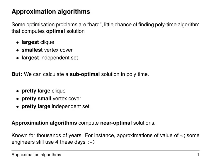
Approximation algorithms

Some optimisation problems are “hard”, little chance of finding poly-time algorithm that computes optimal solution

• largest clique
• smallest vertex cover
• largest independent set

But: We can calculate a sub-optimal solution in poly time.

• pretty large clique
• pretty small vertex cover
• pretty large independent set

Approximation algorithms compute near-optimal solutions. Known for thousands of years. For instance, approximations of value of ⇡; some engineers still use 4 these days :-)

Approximation algorithms 1

Consider optimisation problem. Each potential solution has positive cost, we want near-optimal solution. Depending on problem, optimal solution may be one with

• maximum possible cost (maximisation problem), like maximum clique,
• or one with minimum possible cost (minimisation problem), like minimum

vertex cover. Algorithm has approximation ratio of ⇢(n), if for any input of size n, the cost C

• f its solution is within factor ⇢(n) of cost of optimal solution C⇤, i.e.

max C C⇤, C⇤ C

!

 ⇢(n)

Approximation algorithms 2

Maximisation problems:

• 0 < C  C⇤,
• C⇤/C gives factor by which optimal solution is better than approximate solu-

tion (note: C⇤/C 1 and C/C⇤  1). Minimisation problems:

• 0 < C⇤  C,
• C/C⇤ gives factor by which optimal solution is better than approximate solu-

tion (note C/C⇤ 1 and C⇤/C  1). Approximation ratio is never less than one: C C⇤ < 1 ) C⇤ C > 1

Approximation algorithms 3

Approximation Algorithm

An algorithm with guaranteed approximation ration of ⇢(n) is called a ⇢(n)- approximation algorithm. A 1-approximation algorithm is optimal, and the larger the ratio, the worse the solution.

• For many NP-complete problems, constant-factor approximations exist

(i.e. computed clique is always at least half the size of maximum-size clique),

• sometimes in best known approx ratio grows with n,
• and sometimes even proven lower bounds on ratio (for every approximation

alg, the ratio is at least this and that, unless P = NP).

Approximation algorithms 4

Approximation Scheme

Sometimes the approximation ratio improves when spending more computation time. An approximation scheme for an optimisation problem is an approximation al- gorithm that takes as input an instance plus a parameter ✏ > 0 s.t. for any fixed ✏, the scheme is a (1 + ✏)-approximation (trade-off).

Approximation algorithms 5

PTAS and FPTAS

A scheme is a poly-time approximation scheme (PTAS) if for any fixed ✏ > 0, it runs in time polynomial in input size. Runtime can increase dramatically with decreasing ✏, consider T(n) = n2/✏. ✏ 2 1 1/2 1/4 1/100 n T(n) n n2 n4 n8 n200 101 101 102 104 108 10200 102 102 104 108 1016 10400 103 103 106 1012 1024 10600 104 104 108 1016 1032 10800 We want: if ✏ decreases by constant factor, then running time increases by at most some other constant factor, i.e., running time is polynomial in n and 1/✏. Example: T(n) = (2/✏) · n2, T(n) = (1/✏)2 · n3. Such a scheme is called a fully polynomial-time approximation scheme (FPAS).

Approximation algorithms 6

Example 1: Vertex cover

Problem: given graph G = (V, E), find smallest V 0 ✓ V s.t. if (u, v) 2 E, then u 2 V 0 or v 2 V 0 or both. Decision problem is NP-complete, optimisation problem is at least as hard. Trivial 2-approximation algorithm. APPROX-VERTEX-COVER

1: C ; 2: E0 E 3: while E0 6= ; do 4:

let (u, v) be an arbitrary edge of E0

5:

C C [ {(u, v)}

6:

remove from E0 all edges incident on either u or v

7: end while

Claim: after termination, C is a vertex cover of size at most twice the size of an

• ptimal (smallest) one.

Approximation algorithms 7

Example

Step 3: choose edge (a,b) Step 2: choose edge (d,g) Result, size 6 Optimal result, size 4 a b c d e f g Input graph Step 1: choose edge (c,e) a b c d e f g a b c d e f g a b c d e f g a b c d e f g a b c d e f g

Approximation algorithms 8

• Theorem. APPROX-VERTEX-COVER is a poly-time 2-approximation algorithm.
• Proof. The running time is trivially bounded by O(V E) (at most |E| iterations,

each of complexity at most O(V )). However, O(V + E) can easily be shown. Correctness: C clearly is a vertex cover.

Approximation algorithms 9

Size of the cover: let A denote set of edges that are picked ({(c, e), (d, g), (a, b)} in example).

• In order to cover edges in A, any vertex cover, in particular an optimal cover

C⇤, must include at least one endpoint of each edge in A.

• By construction of the algorithm, no two edges in A share an endpoint (once

edge is picked, all edges incident on either endpoint are removed).

• Therefore, no two edges in A are covered by the same vertex in C⇤, and

|C⇤| |A|.

• When an edge is picked, neither endpoint is already in C, thus

|C| = 2 · |A|. Combining (1) and (2) yields |C| = 2 · |A|  2 · |C⇤| (q.e.d.)

Approximation algorithms 10

Interesting observation: we could prove that size of VC returned by alg is at most twice the size of optimal cover, without knowing the latter. How? We lower-bounded size of optimal cover (|C⇤| |A|). One can show that A is in fact a maximal matching in G.

• The size of any maximal matching is always a lower bound on the size of an
• ptimal vertex cover (each edge has to be covered).
• The alg returns VC whose size is twice the size of the maximal matching A.

Approximation algorithms 11

Example 2: The travelling-salesman problem

Problem: given complete, undirected graph G = (V, E) with non-negative inte- ger cost c(u, v) for each edge, find cheapest hamiltonian cycle of G. Consider two cases: with and without triangle inequality. c satisfies triangle inequality, if it is always cheapest to go directly from some u to some w; going by way of intermediate vertices can’t be less expensive. Related decision problem is NP-complete in both cases.

Approximation algorithms 12

TSP with triangle inequality

We use function MST-PRIM(G, c, r), which computes an MST for G and weight function c, given some arbitrary root r. Input: G = (V, E), c : E ! I R APPROX-TSP-TOUR

1: Select arbitrary v 2 V to be “root” 2: Compute MST T for G and c from root r using

MST-PRIM(G, c, r)

3: Let L be list of vertices visited in pre-order tree walk of T 4: Return the hamiltonian cycle that vistis the vertices in the order L Approximation algorithms 13

a a a a a Set of points, lie in grid MST, root a Pre−order walk Resulting tour, cost ca. 19.1 Optimal tour, cost ca. 14.7 a b c d e f g h a b c d e f g h a b c d e f g h a b c d e f g h a b c d e f g h

Approximation algorithms 14

• Theorem. APPROX-TSP-TOUR is a poly-time 2-approximation algorithm for the

TSP problem with triangle inequality. Proof. Polynomial running time obvious, simple MST-PRIM takes Θ(V 2), computing preorder walk takes no longer. Correctness obvious, preorder walk is always a tour. Approximation ratio: Let H⇤ denote an optimal tour for given set of vertices. Deleting any edge from H⇤ gives a spanning tree. Thus, weight of minimum spanning tree is lower bound on cost of optimal tour: c(T)  c(H⇤)

Approximation algorithms 15

A full walk of T lists vertices when they are first visited, and also when they are returned to, after visiting a subtree. Ex: a,b,c,b,h,b,a,d,e,f,e,g,e,d,a Full walk W traverses every edge exactly twice (although some vertex perhaps way more often), thus c(W) = 2c(T) Together with c(T)  c(H⇤), this gives c(W) = 2c(T)  2c(H⇤)

Approximation algorithms 16

Problem: W is in general not a proper tour, since vertices may be visited more than once. . . But: by our friend, the triangle inequality, we can delete a visit to any vertex from W and cost does not increase. Deleting a vertex v from walk W between visits to u and w means going from u directly to w, without visiting v. This way, we can consecutively remove all multiple visits to any vertex. Ex: full walk a,b,c,b,h,b,a,d,e,f,e,g,e,d,a becomes a,b,c,h,d,e,f,g.

Approximation algorithms 17

This ordering (with multiple visits deleted) is identical to that obtained by preorder walk of T (with each vertex visited only once). It certainly is a Hamiltonian cycle. Let’s call it H. H is just what is computed by APPROX-TSP-TOUR. H is obtained by deleting vertices from W, thus c(H)  c(W) Conclusion: c(H)  c(W)  2c(H⇤) (q.e.d.) Although factor 2 looks nice, there are better algorithms. There’s a 3/2 approximation algorithm by Christofedes (with triangle inequality). Arora and Mitchell have shown that there is a PAS if the points are in the Euclidean plane (meaning the triangle inequality holds).

Approximation algorithms 18

The general TSP

Now c does no longer satisfy triangle inequality.

• Theorem. If P 6= NP, then for any constant ⇢ 1, there is no poly-time ⇢-

approximation algorithm for the general TSP .

• Proof. By contradiction. Suppose there is a poly-time ⇢-approximation algorithm

A, ⇢ 1 integer. We use A to solve HAMILTON-CYCLE in poly time (this implies P = NP). Let G = (V, E) be instance of HAMILTON-CYCLE. Let G0 = (V, E0) the com- plete graph on V : E0 = {(u, v) : u, v 2 V ^ u 6= v} We assign costs to edges in E0: c(u, v) =

(

1 if (u, v) 2 E ⇢ · |V | + 1

• therwise

Creating G0 and c from G certainly possible in poly time.

Approximation algorithms 19

Consider TSP instance hG0, ci. If original graph G has a Hamiltonian cycle H, then c assigns cost of one to reach edge of H, and G0 contains tour of cost |V |. Otherwise, any tour of G0 must contain some edge not in E, thus have cost at least (⇢ · |V | + 1)

| {z }

62E

+ (|V | 1)

| {z }

2E

= ⇢ · |V | + |V | (⇢ + 1) · |V | There is a gap of ⇢ · |V | between cost of tour that is Hamiltonian cycle in G (= |V |) and cost of any other tour. Apply A to hG0, ci. By assumption, A returns tour of cost at most ⇢ times the cost of optimal tour. Thus, if G contains Hamiltonian cycle, A must return it. If G is not Hamiltonian, A returns tour of cost > ⇢ · |V |. We can use A to decide HAMILTON-CYCLE. (q.e.d.)

Approximation algorithms 20

The proof was example of general technique for proving that a problem cannot be approximated well. Suppose given NP-hard problem X, produce minimisation problem Y s.t.

• “yes” instances of X correspond to instances of Y with value at most some

k,

• “no” instances of X correspond to instances of Y with value greater than ⇢k

Then there is no ⇢-approximation algorithm for Y unless P = NP.

Approximation algorithms 21

Set-Covering Problem

Input: A finite set X and a family F of subsets over X. Every x 2 X belongs to at least one F 2 F. Output: A minimum S ⇢ F such that X =

[

F2S

F. We say that such S covers X and x 2 X is covered by S0 ⇢ F if there exists a set Si 2 S0 that contains x. The problem is a generalisation of the vertex cover problem. It has many applications (cover a set of skills with workers,...)

Approximation algorithms 22

We use a simple greedy algorithm to solve approximate the problem. The idea is to add in every round a set S to the solution that covers the largest number of uncovered elements. APPROX-SET-COVER

1: U X 2: S ; 3: while U 6= ; do 4:

Select an Si 2 F that maximzes |Si

T U|

5:

U U Si

6:

S S [ Si

7: end while

The algorithm returns S.

Approximation algorithms 23

Theorem. APPROX-SET-COVER is a poly-time log n-approximation algorithm where n = {max |F| : F 2 F}.

• Proof. The running time is clearly polynomially in |X| and |F|.

Correctness: S clearly is a set cover. Remains to show: S is a log n approximation We will use harmonic numbers: H(d) =

d

X

i=1

1 d. H(0) = 0 and H(d) = O(log d).

Approximation algorithms 24

Analysis

• Let Si be the ith subset selected by APPROX-SET-COVER
• We assign a one to each set Si selected by the algorithm.
• We will distribute the cost evenly over all elements that are covered for the

first time.

• Let cx be the cost assigned to x 2 X. Then

cx = 1 |Si (S1 [ S2 [ · · · [ Si1)|.

• Let C be the cost of APPROX-SET-COVER. Then

C =

X

x2X

cx.

Approximation algorithms 25

Analysis II

• Since each x 2 X is in at least one set S0 2 S⇤ we have

X

S02S⇤

X

x2S0

cx

X

x2X

cx := C

• Hence,

C 

X

S02S⇤

X

x2S0

cx.

• Lemma. For any set F 2 F we have

X

x2F

cx  H(|F|). Using the lemma we get C 

X

S02S⇤

X

x2S0

cx 

X

S02S⇤

H(S0)  C⇤ · H(max{|F| : F 2 F}).

Approximation algorithms 26

• Lemma. For any set F 2 F we have

X

x2F

cx  H(|F|).

• Proof. Consider any set F 2 F and i = 1, 2, . . . C and let

ui = |F (S1 [ S2 [ · · · [ Si1)|. ui is the number of elements in F that are not covered by S1, S2, . . . Si. We also define u0 = |F|. Now let k be the smallest index such that uk = 0. Then ui1 ui and ui1 ui elements of F are covered for the first time by Si (for i = 1, . . . k).

Approximation algorithms 27

We have

X

x2F

cx =

k

X

i=1

(ui1 ui) · 1 |Si (S1 [ S2 [ · · · [ Si1)| Observe that |Si (S1 [ S2 [ · · · [ Si1)| |F (S1 [ S2 [ · · · [ Si1)| = ui. (the alg. chooses Si such that the number of newly covered elements is max.). Hence

X

x2F

cx 

k

X

i=1

(ui1 ui) · 1 ui1

Approximation algorithms 28

X

x2F

cx 

k

X

i=1

(ui1 ui) · 1 ui1 =

k

X

i=1 ui1

X

j=ui+1

1 ui1 

k

X

i=1 ui1

X

j=ui+1

1 j =

k

X

i=1

@

ui1

X

j=1

1 j

ui

X

j=1

1 j

1 A

=

k

X

i=1

H(ui1) H(ui)

• =

H(u0) H(uk) = H(u0) H(0) = H(u0) = H(|F|))

Approximation algorithms 29

Randomised approximation

A randomised algorithm has an approximation ratio of ⇢(n) if, for any input of size n, the expected cost C is within a factor of ⇢(n) of cost C⇤ of optimal solu- tion. max C C⇤, C⇤ C

!

 ⇢(n) So, just like with “standard” algorithm, except the approximation ratio is for the expected cost. Consider 3-CNF-SAT, problem of deciding whether or not a given formula in 3CNF is satisfiable. 3-CNF-SAT is NP-complete. Q: What could be a related optimisation problem?

Approximation algorithms 30

A: MAX-3-CNF Even if some formula is perhaps not satisfiable, we might be interested in satisfy- ing as many clauses as possible. Assumption: each clause consists of exactly three distinct literals, and does not contain both a variable and its negation (so, we can not have x_x_y or x_x_y). Randomised algorithm: Independently, set each variable to 1 with probability 1/2, and to 0 with probability 1/2.

• Theorem. Given an instance of MAX-3-CNF with n variables x1, x2, . . . , xn and

m clauses, the described randomised algorithm is a randomised 8/7-approximation algorithm.

• Proof. Define indicator variables Y1, Y2, . . . , Ym with

Yi =

(

1 clause i is satisfied by the alg’s assignment

• therwise

Approximation algorithms 31

This means Yi = 1 if at least one of the three literals in clause i has been set to 1. By assumption, settings of all three literals are independent. A clause is not satisfied iff all three literals are set to 0, thus P [Yi = 0] =

✓1

2

◆3

= 1 8 and therefore P [Yi = 1] = 1

✓1

2

◆3

= 7 8 and E [Yi] = 0 · P [Yi = 0] + 1 · P [Yi = 1] = P [Yi = 1] = 7 8

Approximation algorithms 32

Let Y be number of satisfied clauses, i.e. Y = Y1 + · · · + Ym. By linearity of expectation, E [Y ] = E

2 4

m

X

i=1

Yi

3 5 =

m

X

i=1

E [Yi] =

m

X

i=1

7 8 = 7 8 · m m is upper bound on number of satisfied clauses, thus approximation ratio is at most m

7 8 · m

= 8 7 (q.e.d.)

Approximation algorithms 33

An approximation scheme

An instance of the SUBSET-SUM problem is a pair hS, ti with S = {x1, x2, . . . , xn} a set of positive integers, and t a positive integer. The decision problem asks whether there is a subset of S that adds up to t. SUBSET-SUM is NP-complete. In the optimisation problem we wish to find a subset of S whose sum is as large as possible but not larger than t. An exponential-time algorithm Just enumerate all subsets of S and pick the one with largest sum that does not exceed t. There are 2n possible subsets (an item is “in” or “out”), so this takes time O(2n).

Approximation algorithms 34

Implementation could look as follows. In iteration i, the alg computes sums of all subsets of {x1, x2, . . . , xi}. As starting point, it uses all sums of subsets of {x1, x2, . . . , xi1}. Once a particular subset S0 has sum exceeding t, no reason to maintain it: no superset of S0 can possibly be a solution. Iteratively compute Li, list of sums of all subsets of {x1, x2, . . . , xi} that do not exceed t. Return the maximum value in Ln. If L is a list of positive integers and x is another positive integer, then L + x denotes list derived from L with each element of L increased by x. Ex: L = h4, 3, 2, 4, 6, 7i, L + 3 = h7, 6, 5, 7, 9, 10i We also use this notation for sets: S + x = {s + x : s 2 S}.

Approximation algorithms 35

Let MERGE-LIST(L, L0) return sorted list that is merge of sorted L and L0 with duplicates removed. Running time is O(|L| + |L0|). EXACT-SUBSET-SUM(S = {x1, x2, . . . , xn}, t)

1: L0 h0i 2: for i 1 to n do 3:

Li MERGE-LIST(Li1, Li1 + xi)

4:

remove from Li every element that is greater than t

5: end for 6: return the largest element in Ln

How does it work? Let Pi denote set of all values that can be obtained by selecting a (possibly empty) subset of {x1, x2, . . . , xi} and summing its members. Ex: S = {1, 4, 5}, then P1 = {0, 1} P2 = {0, 1, 4, 5} P3 = {0, 1, 4, 5, 6, 9, 10}

Approximation algorithms 36

Clearly, Pi = Pi1 [ (Pi1 + xi) Can prove by induction on i that Li is a sorted list containing every element of Pi with value at most t. Length of Li can be 2i, thus EXACT-SUBSET-SUM is an exponential time algorithm in general. However, in special cases it is poly-time if t is polynomial in |S|, or if all xi are polynomial in |S|.

Approximation algorithms 37

A fully-polynomial approximation scheme

Recall: running time must be polynomial in both 1/✏ and n. Basic idea: modify exact exponential time algorithm by trimming each list Li after creation: If two values are “close”, then we don’t maintain both of them (will give similar approximations). Precisely: given “trimming parameter” with 0 < < 1, then from a given list L we remove as many elements as possible, such that if L0 is the result, for every element y that is removed, there is an element z still in L0 that “aproximates” y: y 1 +  z  y Note: “one-sided error” We say z represents y in L0. Each removed y is represented by some z satisfying the condition from above.

Approximation algorithms 38

Example: = 0.1, L = h10, 11, 12, 15, 20, 21, 22, 23, 24, 29i We can trim L to L0 = h10, 12, 15, 20, 23, 29i 11 is represented by 10 21, 22 are represented by 20 24 is represented by 23 Given list L = hy1, y2, . . . , ymi with y1  y2  · · ·  ym, the following function trims L in time Θ(m). TRIM(L, )

1: L0 = hy1i 2: last= y1 3: for i 2 to m do 4:

if yi > last · (1 + ) then

5:

/* yi last because L is sorted */

6:

append yi onto end of L0

7:

last yi

8:

end if

9: end for Approximation algorithms 39

Now we can construct our approximation scheme. Input is S = {x1, x2, . . . , xn}, xi integer, target integer t, and “approximation parameter” ✏ with 0 < ✏ < 1. It will return value z whose value is within 1 + ✏ factor of optimal solution. APPROX-SUBSET-SUM(S = {x1, x2, . . . , xn}, t, ✏)

1: L0 h0i 2: for i 1 to n do 3:

Li MERGE-LIST(Li1, Li1 + xi)

4:

Li TRIM(Li, ✏/2n)

5:

remove from Li every element that is greater than t

6: end for 7: return z⇤, the largest element in Ln Approximation algorithms 40

Example S = {104, 102, 201, 101}, t = 308, ✏ = 0.4 = ✏/2n = 0.4/8 = 0.05 line 1 L0 = h0i 3 L1 = h0, 104i 4 L1 = h0, 104i 5 L1 = h0, 104i 3 L2 = h0, 102, 104, 206i 4 L2 = h0, 102, 206i 5 L2 = h0, 102, 206i 3 L3 = h0, 102, 201, 206, 303, 407i 4 L3 = h0, 102, 201, 303, 407i 5 L3 = h0, 102, 201, 303i 3 L4 = h0, 101, 102, 201, 203, 302, 303, 404i 4 L4 = h0, 101, 201, 302, 404i 5 L4 = h0, 101, 201, 302i Alg returns z⇤ = 302, well within ✏ = 40% of optimal answer 307 = 104 + 102 + 101 (in fact, within 2%).

Approximation algorithms 41

• Theorem. APPROX-SUBSET-SUM is fully polynomial approximation scheme for

the subset-sum problem.

• Proof. Trimming Li and removing from Li every element that is greater than t

maintain property that every element of Li is member of Pi. Thus, z⇤ is sum of some subset of S. Let y⇤ 2 Pn denote an optimal solution. Clearly, z⇤  y⇤ (have removed elements that are too large). Need to show y⇤/z⇤  1 + ✏ and that running time is polynomial in n and 1/✏. Can be shown (by induction) that 8y 2 Pi with y  t there is some z 2 Ln with y (1 + ✏/2n)i  z  y

Approximation algorithms 42

This also holds for y⇤ 2 Pn, thus there is some z 2 Ln with y⇤ (1 + ✏/2n)n  z  y⇤ and therefore y⇤ z 

✓

1 + ✏ 2n

◆n

z⇤ is largest value in Ln, thus y⇤ z⇤ 

✓

1 + ✏ 2n

◆n

Remains to show that y⇤/z⇤  1 + ✏.

Approximation algorithms 43

We know (1 + a/n)n  ea, and therefore

✓

1 + ✏ 2n

◆n

=

✓

1 + ✏ 2n

◆2n·(1/2)

=

✓

1 + ✏ 2n

◆2n!1/2

=

✓

1 + ✏ 2n

◆2n!1/2

 (e✏)1/2 = e✏/2 This, together with e✏/2  1 + ✏/2 + (✏/2)2  1 + ✏ gives y⇤ z⇤ 

✓

1 + ✏ 2n

◆n

 1 + ✏

Approximation algorithms 44

Approximation ratio OK, but what with running time? We derive bound on |Li|, Running time of APPROX-SUBSET-SUM is polynomial in lengths of Li. After trimming, successive elements z and z0 of Li fulfill z0/z > 1 + ✏/2n. Thus, each list contains 0, possibly 1, and at most blog1+✏/2n tc additional values. We have |Li|  (log1+✏/2n t) + 2 = ln t ln(1 + ✏/2n) + 2  2n(1 + ✏/2n) ln t ✏ + 2 /* because of x/(1 + x)  ln(1 + x)  x */  4n ln t ✏ + 2 /* because of 0 < ✏ < 1 */ This is polynomial in size of input (log t bits for t, plus bits for x1, x2, . . . , xn). Thus, it’s polynomial in n and 1/✏.

Approximation algorithms 45

Bin Packing

We are given n items with sizes a1, a2, . . . an with ai 2 (0, 1]. The goal is to pack the items into m bins with capacity 1 each, and, thereby, to minimise the number of used bins. Approximation is clear: find a value that is as close as possible to the optimal value for m.

Approximation algorithms 46

Very easy: 2-approximation

This can be done using the First Fit algorithm:

• consider the items in an arbitrary order
• try to fit item into one of the existing bins, if not possible use a new bin for the

item. Easy to see that it calculates a two-approximation: If the algorithm uses m bins then at least m 1 of them are more than half full. Therefore a1 + a2 + · · · + an m 1 2 . Hence, m 1 < 2 OPT and m  2 OPT.

Approximation algorithms 47

Theorem: For any ✏ > 0, there is no bin packing algorithm having an approxima- tion ratio of 3/2 ✏, unless P = NP.

• Proof. Assume we have such an algorithm, than we can solve the SET PARTI-

TIONING problem.

In SET PARTITIONING, we are given n non-negative numbers a1, a2, . . . , an and we would like to partition them into two sets having sum (a1 + a2 + · · · + an)/2 This is the same than asking: can I pack the elements in two bins of size (a1 + a2 + · · · + an)/2 . A (3/2✏)-approximation algorithm has to optput 2 for an instance of BIN BACK-

ING that can be packed into two bins.

An asymptotic PTAS

Theorem: For any 0 < ✏  1/2, there is an algorithm A✏ that runs in time poly(n) and finds a packing using at most (1 + 2✏) OPT + 1 bins. The proof is split in two parts:

• It is easy to pack small items into bins. Hence, we consider the small items

in the end.

• Only the big items have to be packed well.

Approximation algorithms 49

Big Items

Lemma: Consider an instance I in which all n items have a size of at least ✏. Then there is a poly(n) time (1 + ✏)-approximation. Proof.

• First we sort the items by increasing size.
• Then we partition the items into K = d1/✏2e groups having at most Q =

bn✏2c items. (Note: two groups can have items of the same size!)

• Construct instance J by rounding up the size of each item to the size of the

largest item in the group.

• J has at most K different item sizes. Hence, there is a poly(n) time algorithm

that solves J optimally: – The number of items per bin is bounded by M = b1/✏c. – The number of possible bin types is R =

⇣M+K

M

⌘

(which is constant). – Hence, the number of possible packings is at most P =

⇣n+R

R

⌘

(which is polynomial in n). We can enumerate all of them.

Approximation algorithms 50

• Note: the packing we get is also valid for the original instance I
• To show

OPT(J)  (1 + ✏) · OPT(I). – Consider instance J0 which is defined like J but we round down instead

• f rounding up. Clearly

OPT(J0)  OPT(I). – Instance J0 yields a packing for all items of J (and I) but the Q items of the largest group of J. Hence OPT(J)  OPT(J0) + Q  OPT(I) + Q. – The largest group is packed into at most Q = bn✏2c bins. – We also have (min. item size is ✏) OPT(I) n✏. – We have Q = bn✏2c  ✏ OPT and OPT(J)  (1 + ✏) · OPT(I)

Approximation algorithms 51

Small Items

They can be packed using first fit, the "hole" in every bin is at most ✏.

Approximation algorithms 52

APPROX-BIN-PACKING(I = {a1, a2, . . . , an})

1: Remove items of size < ✏ 2: Round to optain constant number of item sizes 3: Find optimal Packing for the rounded items 4: Use this packing for original item sizes 5: Pack items of size < ✏ using First-Fit Approximation algorithms 53

Back to the Proof of the Theorem.

Let I be the input instance and I0 the set of large items of I. Let M be the number

• f bins used by APPROX-BIN-PACKING.

We can find a packing for I0 using at most (1 + ✏) · OPT(I0) many bins. We pack the small items in First Fit manner into the bins opened for I0 and open new bins if necessary.

• If no new bins are opened we have a M  (1 + ✏) · OPT(I0)  (1 + ✏) ·

OPT(I).

• If new bins are opened for the small items, all but the last bin are full to the

extend of at least 1 ✏. Hence the sum of item sizes in I is at least (M 1)·(1✏) and with ✏  1/2 M  OPT 1 ✏ + 1  (1 + 2✏) · OPT(I) + 1.

Approximation algorithms 54

The Knapsack Problem

Given: A set S = {a1, a2, . . . an} of objects with sizes s1, s2, . . . sn 2 Z+ and profits p1, p2, . . . pn 2 Z+ and a knapsack capacity B. Goal: Find a subset of the objects whose total size is bounded by B and the total profit is maximised. First Idea: Use a simple greedy algorithm that sorts the items by decreasing ratio

• f profit to size and pick objects in that order.

Homework: That algorithm can be arbitrarily bad!

Approximation algorithms 55

Better: APPROX-KNAPSACK(I = {a1, a2, . . . , an})

1: Use the greedy algorithm to find a set of items S 2: Take the best of S and the item with largest profit

Theorem APPROX-KNAPSACK calculates a 2-approximation. Proof. Let k be the index of the first item that is not picked by the greedy algorithm. Then p1 + p2 + · · · + pk OPT(I) (recall Problem Sheet 2) Hence, either p1 + p2 + · · · + pk1 or pk is at least OPT

2

.

Approximation algorithms 56