Polynomial approximation and floating-point numbers Algorithms - PowerPoint PPT Presentation

Scope of my researches Approximation theory Polynomial approximation with floating-point numbers Lattices and LLL algorithm A concrete case Conclusion Focus on polynomial approximation ◮ The definition often gives a natural way to compute approximations of f . For instance : a power series and a formally computed bound on the error. ◮ Remark : a truncated power series is a polynomial ֒ → especially nice to evaluate : it requires only additions and multiplications (fast on modern processors). ◮ Truncated power series are useful but. . . . . . usually inefficient in term of number of operations. ֒ → exp ( x ) on [ − 1 ; 2 ] with an absolute error ≤ 0 . 01 : 7 terms of the series / a degree 4 polynomial is sufficient. ◮ Natural question : what degree should have a polynomial to give a suitable approximation ? Sylvain Chevillard Polynomial approximation and floating-point numbers 6

Scope of my researches Approximation theory Polynomial approximation with floating-point numbers Lattices and LLL algorithm A concrete case Conclusion Reminder of approximation theory ◮ Polynomial approximation theory has been deeply studied since the XIXth century. Sylvain Chevillard Polynomial approximation and floating-point numbers 7

Scope of my researches Approximation theory Polynomial approximation with floating-point numbers Lattices and LLL algorithm A concrete case Conclusion Reminder of approximation theory ◮ Polynomial approximation theory has been deeply studied since the XIXth century. ◮ Th. (Weierstrass) : the set R [ X ] is dense in C ([ a , b ]) . Bernstein gave an effective polynomial sequence. Sylvain Chevillard Polynomial approximation and floating-point numbers 7

Scope of my researches Approximation theory Polynomial approximation with floating-point numbers Lattices and LLL algorithm A concrete case Conclusion Reminder of approximation theory ◮ Polynomial approximation theory has been deeply studied since the XIXth century. ◮ Th. (Weierstrass) : the set R [ X ] is dense in C ([ a , b ]) . Bernstein gave an effective polynomial sequence. ◮ Th. (Chebyshev) : given n and f there is a unique polynomial p of degree ≤ n minimizing � f − p � ∞ . Sylvain Chevillard Polynomial approximation and floating-point numbers 7

Scope of my researches Approximation theory Polynomial approximation with floating-point numbers Lattices and LLL algorithm A concrete case Conclusion Reminder of approximation theory (2) ◮ Th. (Chebyshev) : characterization of the optimal error. n + 2 oscillations Sylvain Chevillard Polynomial approximation and floating-point numbers 8

Scope of my researches Approximation theory Polynomial approximation with floating-point numbers Lattices and LLL algorithm A concrete case Conclusion Reminder of approximation theory (2) ◮ Th. (Chebyshev) : characterization of the optimal error. ◮ Th. (La Vallée Poussin) : links the quality of an approximation with its error function. Sylvain Chevillard Polynomial approximation and floating-point numbers 8

Scope of my researches Approximation theory Polynomial approximation with floating-point numbers Lattices and LLL algorithm A concrete case Conclusion Reminder of approximation theory (2) ◮ Th. (Chebyshev) : characterization of the optimal error. ◮ Th. (La Vallée Poussin) : links the quality of an approximation with its error function. ◮ Remez’ algorithm : given n , computes the optimal polynomial of degree ≤ n (called minimax). Sylvain Chevillard Polynomial approximation and floating-point numbers 8

Scope of my researches Approximation theory Polynomial approximation with floating-point numbers Lattices and LLL algorithm A concrete case Conclusion Representing real numbers in computers ◮ In general a real number is not finitely representable. ֒ → one has to choose a subset S and approximate the real line by the elements of S . Sylvain Chevillard Polynomial approximation and floating-point numbers 9

Scope of my researches Approximation theory Polynomial approximation with floating-point numbers Lattices and LLL algorithm A concrete case Conclusion Representing real numbers in computers ◮ In general a real number is not finitely representable. ֒ → one has to choose a subset S and approximate the real line by the elements of S . ◮ A usual choice : floating-point numbers (IEEE-754 standard). Sylvain Chevillard Polynomial approximation and floating-point numbers 9

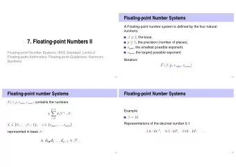
Scope of my researches Approximation theory Polynomial approximation with floating-point numbers Lattices and LLL algorithm A concrete case Conclusion Representing real numbers in computers ◮ In general a real number is not finitely representable. ֒ → one has to choose a subset S and approximate the real line by the elements of S . ◮ A usual choice : floating-point numbers (IEEE-754 standard). ◮ A floating-point number with radix β and precision t is a number of the form m · β e where : ◮ m ∈ Z is the mantissa and is written with exactly t digits ; ◮ e ∈ Z is the exponent. It is usually bounded in a range [ e min , e max ] . Sylvain Chevillard Polynomial approximation and floating-point numbers 9

Scope of my researches Approximation theory Polynomial approximation with floating-point numbers Lattices and LLL algorithm A concrete case Conclusion Representing real numbers in computers ◮ In general a real number is not finitely representable. ֒ → one has to choose a subset S and approximate the real line by the elements of S . ◮ A usual choice : floating-point numbers (IEEE-754 standard). ◮ A floating-point number with radix β and precision t is a number of the form m · β e where : ◮ m ∈ Z is the mantissa and is written with exactly t digits ; ◮ e ∈ Z is the exponent. It is usually bounded in a range [ e min , e max ] . ◮ IEEE double format : β = 2, t = 53, and e ∈ � − 1074 , 971 � . Sylvain Chevillard Polynomial approximation and floating-point numbers 9

Scope of my researches Approximation theory Polynomial approximation with floating-point numbers Lattices and LLL algorithm A concrete case Conclusion Representing real numbers in computers ◮ In general a real number is not finitely representable. ֒ → one has to choose a subset S and approximate the real line by the elements of S . ◮ A usual choice : floating-point numbers (IEEE-754 standard). ◮ A floating-point number with radix β and precision t is a number of the form m · β e where : ◮ m ∈ Z is the mantissa and is written with exactly t digits ; ◮ e ∈ Z is the exponent. It is usually bounded in a range [ e min , e max ] . ◮ IEEE double format : β = 2, t = 53, and e ∈ � − 1074 , 971 � . ◮ From now on, we will assume that [ e min , e max ] = [ −∞ , + ∞ ] . Sylvain Chevillard Polynomial approximation and floating-point numbers 9

Scope of my researches Approximation theory Polynomial approximation with floating-point numbers Lattices and LLL algorithm A concrete case Conclusion Polynomials with floating-point coefficients ◮ Each coefficient of a polynomial is represented by a floating-point number. Sylvain Chevillard Polynomial approximation and floating-point numbers 10

Scope of my researches Approximation theory Polynomial approximation with floating-point numbers Lattices and LLL algorithm A concrete case Conclusion Polynomials with floating-point coefficients ◮ Each coefficient of a polynomial is represented by a floating-point number. ◮ Naive method to obtain a polynomial approximation of f : ◮ compute the real minimax p ∗ ; ◮ replace each coefficient a i of p ∗ by the nearest floating-point number � a i ; ◮ use � a n X n . p = � a 0 + � a 1 X + · · · + � Sylvain Chevillard Polynomial approximation and floating-point numbers 10

Scope of my researches Approximation theory Polynomial approximation with floating-point numbers Lattices and LLL algorithm A concrete case Conclusion Polynomials with floating-point coefficients ◮ Each coefficient of a polynomial is represented by a floating-point number. ◮ Naive method to obtain a polynomial approximation of f : ◮ compute the real minimax p ∗ ; ◮ replace each coefficient a i of p ∗ by the nearest floating-point number � a i ; ◮ use � a n X n . p = � a 0 + � a 1 X + · · · + � ◮ � p may be far from being optimal. Sylvain Chevillard Polynomial approximation and floating-point numbers 10

Scope of my researches Approximation theory Polynomial approximation with floating-point numbers Lattices and LLL algorithm A concrete case Conclusion Polynomials with floating-point coefficients ◮ Each coefficient of a polynomial is represented by a floating-point number. ◮ Naive method to obtain a polynomial approximation of f : ◮ compute the real minimax p ∗ ; ◮ replace each coefficient a i of p ∗ by the nearest floating-point number � a i ; ◮ use � a n X n . p = � a 0 + � a 1 X + · · · + � ◮ � p may be far from being optimal. ◮ Example with f ( x ) = log 2 ( 1 + 2 − x ) , n = 6, on [ 0 ; 1 ] with single precision coefficients (24 bits). Minimax Naive method Optimal 8 . 3 · 10 − 10 119 · 10 − 10 10 . 06 · 10 − 10 Sylvain Chevillard Polynomial approximation and floating-point numbers 10

Scope of my researches Approximation theory Polynomial approximation with floating-point numbers Lattices and LLL algorithm A concrete case Conclusion Previous works ◮ W. Kahan claims to have studied the question and proposed an efficient method. No published work, no draft. Sylvain Chevillard Polynomial approximation and floating-point numbers 11

Scope of my researches Approximation theory Polynomial approximation with floating-point numbers Lattices and LLL algorithm A concrete case Conclusion Previous works ◮ W. Kahan claims to have studied the question and proposed an efficient method. No published work, no draft. ◮ D. Kodek has studied a similar problem in signal processing. Limited to small precision and degree (typically t < 10 , n < 20). Sylvain Chevillard Polynomial approximation and floating-point numbers 11

Scope of my researches Approximation theory Polynomial approximation with floating-point numbers Lattices and LLL algorithm A concrete case Conclusion Previous works ◮ W. Kahan claims to have studied the question and proposed an efficient method. No published work, no draft. ◮ D. Kodek has studied a similar problem in signal processing. Limited to small precision and degree (typically t < 10 , n < 20). ◮ N. Brisebarre, J.-M. Muller and A. Tisserand have proposed an approach by linear programming (the implementation relies on P. Feautrier’s tool PIP). Sylvain Chevillard Polynomial approximation and floating-point numbers 11

Scope of my researches Approximation theory Polynomial approximation with floating-point numbers Lattices and LLL algorithm A concrete case Conclusion Method of Brisebarre, Muller and Tisserand ◮ Idea : they reduce the initial problem to the problem of finding the points with integer coordinates in a polytope of R n + 1 . Sylvain Chevillard Polynomial approximation and floating-point numbers 12

Scope of my researches Approximation theory Polynomial approximation with floating-point numbers Lattices and LLL algorithm A concrete case Conclusion Method of Brisebarre, Muller and Tisserand ◮ Idea : they reduce the initial problem to the problem of finding the points with integer coordinates in a polytope of R n + 1 . ◮ This approach is certified. . . Sylvain Chevillard Polynomial approximation and floating-point numbers 12

Scope of my researches Approximation theory Polynomial approximation with floating-point numbers Lattices and LLL algorithm A concrete case Conclusion Method of Brisebarre, Muller and Tisserand ◮ Idea : they reduce the initial problem to the problem of finding the points with integer coordinates in a polytope of R n + 1 . ◮ This approach is certified. . . ◮ . . . and flexible (may be used to find real minimax, constrained real minimax, polynomial with floating-point coefficients, odd polynomials, etc.). Sylvain Chevillard Polynomial approximation and floating-point numbers 12

Scope of my researches Approximation theory Polynomial approximation with floating-point numbers Lattices and LLL algorithm A concrete case Conclusion Method of Brisebarre, Muller and Tisserand ◮ Idea : they reduce the initial problem to the problem of finding the points with integer coordinates in a polytope of R n + 1 . ◮ This approach is certified. . . ◮ . . . and flexible (may be used to find real minimax, constrained real minimax, polynomial with floating-point coefficients, odd polynomials, etc.). ◮ But : ◮ its time is exponential ; Sylvain Chevillard Polynomial approximation and floating-point numbers 12

Scope of my researches Approximation theory Polynomial approximation with floating-point numbers Lattices and LLL algorithm A concrete case Conclusion Method of Brisebarre, Muller and Tisserand ◮ Idea : they reduce the initial problem to the problem of finding the points with integer coordinates in a polytope of R n + 1 . ◮ This approach is certified. . . ◮ . . . and flexible (may be used to find real minimax, constrained real minimax, polynomial with floating-point coefficients, odd polynomials, etc.). ◮ But : ◮ its time is exponential ; ◮ it is very sensitive to some parameters. Sylvain Chevillard Polynomial approximation and floating-point numbers 12

Scope of my researches Approximation theory Polynomial approximation with floating-point numbers Lattices and LLL algorithm A concrete case Conclusion Method of Brisebarre, Muller and Tisserand ◮ Idea : they reduce the initial problem to the problem of finding the points with integer coordinates in a polytope of R n + 1 . ◮ This approach is certified. . . ◮ . . . and flexible (may be used to find real minimax, constrained real minimax, polynomial with floating-point coefficients, odd polynomials, etc.). ◮ But : ◮ its time is exponential ; ◮ it is very sensitive to some parameters. ◮ We developed a new method : ◮ fast (it is proven to run in polynomial time) ; ◮ heuristic (there is no proof that the result is always tight) ; ◮ with good practical results. Sylvain Chevillard Polynomial approximation and floating-point numbers 12

Scope of my researches Approximation theory Polynomial approximation with floating-point numbers Lattices and LLL algorithm A concrete case Conclusion Formalization of the problem ◮ Problem : given n and a floating-point format, find (one of) the polynomial(s) p of degree ≤ n with floating-point coefficients minimizing � p − f � ∞ . Sylvain Chevillard Polynomial approximation and floating-point numbers 13

Scope of my researches Approximation theory Polynomial approximation with floating-point numbers Lattices and LLL algorithm A concrete case Conclusion Formalization of the problem ◮ Problem : given n and a floating-point format, find (one of) the polynomial(s) p of degree ≤ n with floating-point coefficients minimizing � p − f � ∞ . ◮ Remark : the existence is still ensured. The unicity may be lost. Sylvain Chevillard Polynomial approximation and floating-point numbers 13

Scope of my researches Approximation theory Polynomial approximation with floating-point numbers Lattices and LLL algorithm A concrete case Conclusion Formalization of the problem ◮ Problem : given n and a floating-point format, find (one of) the polynomial(s) p of degree ≤ n with floating-point coefficients minimizing � p − f � ∞ . ◮ Remark : the existence is still ensured. The unicity may be lost. ◮ A simplification : we may try to guess the value of each e i (assuming that the coefficients of p and p ∗ have the same order of magnitude) ֒ → if e i is correctly guessed, we are reduced to find m i ∈ Z such that � � � � n � � � m i · β e i x i � f ( x ) − � � � i = 0 ∞ is minimal. Sylvain Chevillard Polynomial approximation and floating-point numbers 13

Scope of my researches Approximation theory Polynomial approximation with floating-point numbers Lattices and LLL algorithm A concrete case Conclusion Description of our method Our goal : find p approximating f and with the following form : m 0 · β e 0 + m 1 · β e 1 X + · · · + m n · β e n X n Sylvain Chevillard Polynomial approximation and floating-point numbers 14

Scope of my researches Approximation theory Polynomial approximation with floating-point numbers Lattices and LLL algorithm A concrete case Conclusion Description of our method Our goal : find p approximating f and with the following form : m 0 · β e 0 + m 1 · β e 1 X + · · · + m n · β e n X n ◮ We use the idea of interpolation : Sylvain Chevillard Polynomial approximation and floating-point numbers 14

Scope of my researches Approximation theory Polynomial approximation with floating-point numbers Lattices and LLL algorithm A concrete case Conclusion Description of our method Our goal : find p approximating f and with the following form : m 0 · β e 0 + m 1 · β e 1 X + · · · + m n · β e n X n ◮ We use the idea of interpolation : ◮ we choose n + 1 points x 0 , · · · , x n in [ a , b ] ; Sylvain Chevillard Polynomial approximation and floating-point numbers 14

Scope of my researches Approximation theory Polynomial approximation with floating-point numbers Lattices and LLL algorithm A concrete case Conclusion Description of our method Our goal : find p approximating f and with the following form : m 0 · β e 0 + m 1 · β e 1 X + · · · + m n · β e n X n ◮ We use the idea of interpolation : ◮ we choose n + 1 points x 0 , · · · , x n in [ a , b ] ; ◮ we search m 0 , · · · , m n such that for all i p ( x i ) = m 0 · β e 0 + m 1 · β e 1 x i + · · · + m n · β e n x n i ≃ f ( x i ) . Sylvain Chevillard Polynomial approximation and floating-point numbers 14

Scope of my researches Approximation theory Polynomial approximation with floating-point numbers Lattices and LLL algorithm A concrete case Conclusion Description of our method Our goal : find p approximating f and with the following form : m 0 · β e 0 + m 1 · β e 1 X + · · · + m n · β e n X n ◮ We use the idea of interpolation : ◮ we choose n + 1 points x 0 , · · · , x n in [ a , b ] ; ◮ we search m 0 , · · · , m n such that for all i p ( x i ) = m 0 · β e 0 + m 1 · β e 1 x i + · · · + m n · β e n x n i ≃ f ( x i ) . ◮ Rewritten with vectors :       β e n · x n β e 0 f ( x 0 ) 0 β e n · x n  β e 0      f ( x 1 )       1 m 0  + · · · + m n ≃ .  .   .   .  . . .      . . . β e n · x n β e 0 f ( x n ) n � �� � � �� � Γ of the form Z − → b 0 + Z − → b 1 + ··· + Z − → − → t ∈ R n + 1 b n Sylvain Chevillard Polynomial approximation and floating-point numbers 14

Scope of my researches Approximation theory Polynomial approximation with floating-point numbers Lattices and LLL algorithm A concrete case Conclusion Notions about lattices Let ( − → b 1 , · · · , − → b n ) be a basis of a real vector space. Sylvain Chevillard Polynomial approximation and floating-point numbers 15

Scope of my researches Approximation theory Polynomial approximation with floating-point numbers Lattices and LLL algorithm A concrete case Conclusion Notions about lattices Let ( − → b 1 , · · · , − → b n ) be a basis of a real vector space. The set of all integer combinations of the − → b i is called a lattice : Γ = Z − → b 1 + Z − → b 2 + · · · + Z − → b n . Sylvain Chevillard Polynomial approximation and floating-point numbers 15

Scope of my researches Approximation theory Polynomial approximation with floating-point numbers Lattices and LLL algorithm A concrete case Conclusion Notions about lattices Let ( − → b 1 , · · · , − → b n ) be a basis of a real vector space. The set of all integer combinations of the − → b i is called a lattice : Γ = Z − → b 1 + Z − → b 2 + · · · + Z − → b n . In general, a lattice has infinitely many bases. Sylvain Chevillard Polynomial approximation and floating-point numbers 15

Scope of my researches Approximation theory Polynomial approximation with floating-point numbers Lattices and LLL algorithm A concrete case Conclusion Notions about lattices Let ( − → b 1 , · · · , − → b n ) be a basis of a real vector space. The set of all integer combinations of the − → b i is called a lattice : Γ = Z − → b 1 + Z − → b 2 + · · · + Z − → b n . In general, a lattice has infinitely many bases. Sylvain Chevillard Polynomial approximation and floating-point numbers 15

Scope of my researches Approximation theory Polynomial approximation with floating-point numbers Lattices and LLL algorithm A concrete case Conclusion Notions about lattices Let ( − → b 1 , · · · , − → b n ) be a basis of a real vector space. The set of all integer combinations of the − → b i is called a lattice : Γ = Z − → b 1 + Z − → b 2 + · · · + Z − → b n . In general, a lattice has infinitely many bases. Sylvain Chevillard Polynomial approximation and floating-point numbers 15

Scope of my researches Approximation theory Polynomial approximation with floating-point numbers Lattices and LLL algorithm A concrete case Conclusion Algorithmic problems In the following we consider the euclidean norm on R n : n � �− → x � 2 = x 2 i . i = 1 ◮ Shortest vector problem (SVP). Sylvain Chevillard Polynomial approximation and floating-point numbers 16

Scope of my researches Approximation theory Polynomial approximation with floating-point numbers Lattices and LLL algorithm A concrete case Conclusion Algorithmic problems In the following we consider the euclidean norm on R n : n � �− → x � 2 = x 2 i . i = 1 ◮ Shortest vector problem (SVP). ◮ Ajtai (1997) and Micciancio (1998) showed that SVP is NP-hard under probabilistic randomized reduction ; it is √ NP-hard to approximate SVP within a factor 2. Sylvain Chevillard Polynomial approximation and floating-point numbers 16

Scope of my researches Approximation theory Polynomial approximation with floating-point numbers Lattices and LLL algorithm A concrete case Conclusion Algorithmic problems In the following we consider the euclidean norm on R n : n � �− → x � 2 = x 2 i . i = 1 ◮ Shortest vector problem (SVP). ◮ Ajtai (1997) and Micciancio (1998) showed that SVP is NP-hard under probabilistic randomized reduction ; it is √ NP-hard to approximate SVP within a factor 2. ◮ There is no polynomial algorithm known to approximate SVP within a factor f ( n ) where f is a polynomial. Sylvain Chevillard Polynomial approximation and floating-point numbers 16

Scope of my researches Approximation theory Polynomial approximation with floating-point numbers Lattices and LLL algorithm A concrete case Conclusion Algorithmic problems In the following we consider the euclidean norm on R n : n � �− → x � 2 = x 2 i . i = 1 ◮ Shortest vector problem (SVP). ◮ Ajtai (1997) and Micciancio (1998) showed that SVP is NP-hard under probabilistic randomized reduction ; it is √ NP-hard to approximate SVP within a factor 2. ◮ There is no polynomial algorithm known to approximate SVP within a factor f ( n ) where f is a polynomial. ◮ Shortest basis problem (SBP). ◮ Given a basis of a lattice L , find a basis ( b 1 , · · · , b n ) of L for which � b 1 � · � b 2 � · · · � b n � is minimal. Sylvain Chevillard Polynomial approximation and floating-point numbers 16

Scope of my researches Approximation theory Polynomial approximation with floating-point numbers Lattices and LLL algorithm A concrete case Conclusion Algorithmic problems In the following we consider the euclidean norm on R n : n � �− → x � 2 = x 2 i . i = 1 ◮ Shortest vector problem (SVP). ◮ Ajtai (1997) and Micciancio (1998) showed that SVP is NP-hard under probabilistic randomized reduction ; it is √ NP-hard to approximate SVP within a factor 2. ◮ There is no polynomial algorithm known to approximate SVP within a factor f ( n ) where f is a polynomial. ◮ Shortest basis problem (SBP). ◮ Given a basis of a lattice L , find a basis ( b 1 , · · · , b n ) of L for which � b 1 � · � b 2 � · · · � b n � is minimal. ◮ It is NP-hard. Sylvain Chevillard Polynomial approximation and floating-point numbers 16

Scope of my researches Approximation theory Polynomial approximation with floating-point numbers Lattices and LLL algorithm A concrete case Conclusion Algorithmic problems ◮ Closest vector problem (CVP). Sylvain Chevillard Polynomial approximation and floating-point numbers 17

Scope of my researches Approximation theory Polynomial approximation with floating-point numbers Lattices and LLL algorithm A concrete case Conclusion Algorithmic problems ◮ Closest vector problem (CVP). Sylvain Chevillard Polynomial approximation and floating-point numbers 17

Scope of my researches Approximation theory Polynomial approximation with floating-point numbers Lattices and LLL algorithm A concrete case Conclusion Algorithmic problems ◮ Closest vector problem (CVP). Sylvain Chevillard Polynomial approximation and floating-point numbers 17

Scope of my researches Approximation theory Polynomial approximation with floating-point numbers Lattices and LLL algorithm A concrete case Conclusion Algorithmic problems ◮ Closest vector problem (CVP). ◮ Emde Boas (1981) : CVP is NP-hard. Sylvain Chevillard Polynomial approximation and floating-point numbers 17

Scope of my researches Approximation theory Polynomial approximation with floating-point numbers Lattices and LLL algorithm A concrete case Conclusion Algorithmic problems ◮ Closest vector problem (CVP). ◮ Emde Boas (1981) : CVP is NP-hard. ◮ Goldreich and al. : CVP is not easier than SVP. Sylvain Chevillard Polynomial approximation and floating-point numbers 17

Scope of my researches Approximation theory Polynomial approximation with floating-point numbers Lattices and LLL algorithm A concrete case Conclusion LLL algorithm ◮ Algorithm developed by A. K. Lenstra, H. W. Lenstra Jr. and L. Lovász. Factoring Polynomials with Rational Coefficients , Math. Annalen 261 , 515-534, 1982. Sylvain Chevillard Polynomial approximation and floating-point numbers 18

Scope of my researches Approximation theory Polynomial approximation with floating-point numbers Lattices and LLL algorithm A concrete case Conclusion LLL algorithm ◮ Algorithm developed by A. K. Lenstra, H. W. Lenstra Jr. and L. Lovász. Factoring Polynomials with Rational Coefficients , Math. Annalen 261 , 515-534, 1982. ◮ Given a basis ( b 1 , . . . , b n ) of a lattice, the LLL algorithm gives a basis ( c 1 , . . . , c n ) composed of pretty short vectors. Sylvain Chevillard Polynomial approximation and floating-point numbers 18

Scope of my researches Approximation theory Polynomial approximation with floating-point numbers Lattices and LLL algorithm A concrete case Conclusion LLL algorithm ◮ Algorithm developed by A. K. Lenstra, H. W. Lenstra Jr. and L. Lovász. Factoring Polynomials with Rational Coefficients , Math. Annalen 261 , 515-534, 1982. ◮ Given a basis ( b 1 , . . . , b n ) of a lattice, the LLL algorithm gives a basis ( c 1 , . . . , c n ) composed of pretty short vectors. → || c 1 || ≤ 2 ( n − 1 ) / 2 λ 1 ( L ) where λ 1 ( L ) denotes the norm of a ֒ shortest nonzero vector of L . ◮ LLL terminates in at most O ( n 6 ln 3 B ) operations with B = max || b i || 2 . Sylvain Chevillard Polynomial approximation and floating-point numbers 18

Scope of my researches Approximation theory Polynomial approximation with floating-point numbers Lattices and LLL algorithm A concrete case Conclusion LLL algorithm ◮ Algorithm developed by A. K. Lenstra, H. W. Lenstra Jr. and L. Lovász. Factoring Polynomials with Rational Coefficients , Math. Annalen 261 , 515-534, 1982. ◮ Given a basis ( b 1 , . . . , b n ) of a lattice, the LLL algorithm gives a basis ( c 1 , . . . , c n ) composed of pretty short vectors. → || c 1 || ≤ 2 ( n − 1 ) / 2 λ 1 ( L ) where λ 1 ( L ) denotes the norm of a ֒ shortest nonzero vector of L . ◮ LLL terminates in at most O ( n 6 ln 3 B ) operations with B = max || b i || 2 . ◮ Very good practical results compared to the theoretical bounds. Sylvain Chevillard Polynomial approximation and floating-point numbers 18

Scope of my researches Approximation theory Polynomial approximation with floating-point numbers Lattices and LLL algorithm A concrete case Conclusion LLL reduction ◮ Gram-Schmidt orthogonalization : to any basis ( b 1 , · · · , b n ) of a vector space is associated an orthogonal basis ( b ∗ 1 , · · · , b ∗ n ) such that Span ( b 1 , · · · , b j ) = Span ( b ∗ 1 , · · · , b ∗ j ) for all j . Sylvain Chevillard Polynomial approximation and floating-point numbers 19

Scope of my researches Approximation theory Polynomial approximation with floating-point numbers Lattices and LLL algorithm A concrete case Conclusion LLL reduction ◮ Gram-Schmidt orthogonalization : to any basis ( b 1 , · · · , b n ) of a vector space is associated an orthogonal basis ( b ∗ 1 , · · · , b ∗ n ) such that Span ( b 1 , · · · , b j ) = Span ( b ∗ 1 , · · · , b ∗ j ) for all j . Remark : one may choose it so that b 1 = b ∗ 1 . Sylvain Chevillard Polynomial approximation and floating-point numbers 19

Scope of my researches Approximation theory Polynomial approximation with floating-point numbers Lattices and LLL algorithm A concrete case Conclusion LLL reduction ◮ Gram-Schmidt orthogonalization : to any basis ( b 1 , · · · , b n ) of a vector space is associated an orthogonal basis ( b ∗ 1 , · · · , b ∗ n ) such that Span ( b 1 , · · · , b j ) = Span ( b ∗ 1 , · · · , b ∗ j ) for all j . Remark : one may choose it so that b 1 = b ∗ 1 . ◮ Prop. : if ( b 1 , · · · , b n ) is the basis of a lattice L , λ 1 ( L ) ≥ min � b ∗ j � . Sylvain Chevillard Polynomial approximation and floating-point numbers 19

Scope of my researches Approximation theory Polynomial approximation with floating-point numbers Lattices and LLL algorithm A concrete case Conclusion LLL reduction ◮ Gram-Schmidt orthogonalization : to any basis ( b 1 , · · · , b n ) of a vector space is associated an orthogonal basis ( b ∗ 1 , · · · , b ∗ n ) such that Span ( b 1 , · · · , b j ) = Span ( b ∗ 1 , · · · , b ∗ j ) for all j . Remark : one may choose it so that b 1 = b ∗ 1 . ◮ Prop. : if ( b 1 , · · · , b n ) is the basis of a lattice L , λ 1 ( L ) ≥ min � b ∗ j � . ◮ Idea of LLL algorithm : control the Gram-Schmidt basis to make b ∗ 1 = b 1 minimal among the vectors of the orthogonal basis. Sylvain Chevillard Polynomial approximation and floating-point numbers 19

Scope of my researches Approximation theory Polynomial approximation with floating-point numbers Lattices and LLL algorithm A concrete case Conclusion LLL reduction ◮ Gram-Schmidt orthogonalization : to any basis ( b 1 , · · · , b n ) of a vector space is associated an orthogonal basis ( b ∗ 1 , · · · , b ∗ n ) such that Span ( b 1 , · · · , b j ) = Span ( b ∗ 1 , · · · , b ∗ j ) for all j . Remark : one may choose it so that b 1 = b ∗ 1 . ◮ Prop. : if ( b 1 , · · · , b n ) is the basis of a lattice L , λ 1 ( L ) ≥ min � b ∗ j � . ◮ Idea of LLL algorithm : control the Gram-Schmidt basis to make b ∗ 1 = b 1 minimal among the vectors of the orthogonal basis. ◮ Babai’s algorithm uses the LLL algorithm to solve an approximation of CVP. Sylvain Chevillard Polynomial approximation and floating-point numbers 19

Scope of my researches Approximation theory Polynomial approximation with floating-point numbers Lattices and LLL algorithm A concrete case Conclusion A concrete case ◮ Example coming from a collaboration with John Harrison from Intel. Sylvain Chevillard Polynomial approximation and floating-point numbers 20

Scope of my researches Approximation theory Polynomial approximation with floating-point numbers Lattices and LLL algorithm A concrete case Conclusion A concrete case ◮ Example coming from a collaboration with John Harrison from Intel. ◮ He asked for a polynomial minimizing the absolute error ◮ approximating f : x �→ 2 x − 1 x ◮ on [ − 1 / 16 , 1 / 16 ] ◮ with a degree 9 polynomial. Sylvain Chevillard Polynomial approximation and floating-point numbers 20

Scope of my researches Approximation theory Polynomial approximation with floating-point numbers Lattices and LLL algorithm A concrete case Conclusion A concrete case ◮ Example coming from a collaboration with John Harrison from Intel. ◮ He asked for a polynomial minimizing the absolute error ◮ approximating f : x �→ 2 x − 1 x ◮ on [ − 1 / 16 , 1 / 16 ] ◮ with a degree 9 polynomial. ◮ a degree 0 coefficient of the form : a 0 h + a 0 l where a 0 h and a 0 l are double extended numbers ◮ other coefficients are double extended numbers. ◮ A double extended number has 64 bits of mantissa. Sylvain Chevillard Polynomial approximation and floating-point numbers 20

Scope of my researches Approximation theory Polynomial approximation with floating-point numbers Lattices and LLL algorithm A concrete case Conclusion A concrete case ◮ Example coming from a collaboration with John Harrison from Intel. ◮ He asked for a polynomial minimizing the absolute error ◮ approximating f : x �→ 2 x − 1 x ◮ on [ − 1 / 16 , 1 / 16 ] ◮ with a degree 9 polynomial. ◮ a degree 0 coefficient of the form : a 0 h + a 0 l where a 0 h and a 0 l are double extended numbers ◮ other coefficients are double extended numbers. ◮ A double extended number has 64 bits of mantissa. ◮ He actually wants to have approximately 74 correct bits. (i.e. ε ≃ 5 . 30 e − 23) Sylvain Chevillard Polynomial approximation and floating-point numbers 20

Scope of my researches Approximation theory Polynomial approximation with floating-point numbers Lattices and LLL algorithm A concrete case Conclusion First try Target Degree 8 minimax Degree 9 minimax 5 . 30 e − 23 40 . 1 e − 23 0 . 07897 e − 23 ֒ → degree 9 should be a good choice. Sylvain Chevillard Polynomial approximation and floating-point numbers 21

Scope of my researches Approximation theory Polynomial approximation with floating-point numbers Lattices and LLL algorithm A concrete case Conclusion First try Target Degree 8 minimax Degree 9 minimax 5 . 30 e − 23 40 . 1 e − 23 0 . 07897 e − 23 ֒ → degree 9 should be a good choice. ◮ How to choose the points ? Sylvain Chevillard Polynomial approximation and floating-point numbers 21

Scope of my researches Approximation theory Polynomial approximation with floating-point numbers Lattices and LLL algorithm A concrete case Conclusion First try Target Degree 8 minimax Degree 9 minimax 5 . 30 e − 23 40 . 1 e − 23 0 . 07897 e − 23 ֒ → degree 9 should be a good choice. ◮ How to choose the points ? ◮ We need n + 1 points. Sylvain Chevillard Polynomial approximation and floating-point numbers 21

Scope of my researches Approximation theory Polynomial approximation with floating-point numbers Lattices and LLL algorithm A concrete case Conclusion First try Target Degree 8 minimax Degree 9 minimax 5 . 30 e − 23 40 . 1 e − 23 0 . 07897 e − 23 ֒ → degree 9 should be a good choice. ◮ How to choose the points ? ◮ We need n + 1 points. ◮ They should correspond to the interpolation intuition. Sylvain Chevillard Polynomial approximation and floating-point numbers 21

Scope of my researches Approximation theory Polynomial approximation with floating-point numbers Lattices and LLL algorithm A concrete case Conclusion First try Target Degree 8 minimax Degree 9 minimax 5 . 30 e − 23 40 . 1 e − 23 0 . 07897 e − 23 ֒ → degree 9 should be a good choice. ◮ How to choose the points ? ◮ We need n + 1 points. ◮ They should correspond to the interpolation intuition. ◮ Chebyshev’s theorem gives n + 1 such points. Sylvain Chevillard Polynomial approximation and floating-point numbers 21

Scope of my researches Approximation theory Polynomial approximation with floating-point numbers Lattices and LLL algorithm A concrete case Conclusion First try : results Target Degree 9 minimax our polynomial p 1 naive method 5 . 30 e − 23 0 . 07897 e − 23 5 . 32 e − 23 40.35 e - 23 Sylvain Chevillard Polynomial approximation and floating-point numbers 22

Scope of my researches Approximation theory Polynomial approximation with floating-point numbers Lattices and LLL algorithm A concrete case Conclusion First try : results Target Degree 9 minimax our polynomial p 1 naive method 5 . 30 e − 23 0 . 07897 e − 23 5 . 32 e − 23 40.35 e - 23 ֒ → pretty good but. . . ◮ Our polynomial does not respect the interpolation constraint. Sylvain Chevillard Polynomial approximation and floating-point numbers 22

Scope of my researches Approximation theory Polynomial approximation with floating-point numbers Lattices and LLL algorithm A concrete case Conclusion First try : results Target Degree 9 minimax our polynomial p 1 naive method 5 . 30 e − 23 0 . 07897 e − 23 5 . 32 e − 23 40.35 e - 23 ֒ → pretty good but. . . ◮ Our polynomial does not respect the interpolation constraint. ◮ degree 1 coefficient of p 1 : a 1 = ◦ ( log ( 2 ) 2 / 2 ) Sylvain Chevillard Polynomial approximation and floating-point numbers 22

Scope of my researches Approximation theory Polynomial approximation with floating-point numbers Lattices and LLL algorithm A concrete case Conclusion First try : results Target Degree 9 minimax our polynomial p 1 naive method 5 . 30 e − 23 0 . 07897 e − 23 5 . 32 e − 23 40.35 e - 23 ֒ → pretty good but. . . ◮ Our polynomial does not respect the interpolation constraint. ◮ degree 1 coefficient of p 1 : a 1 = ◦ ( log ( 2 ) 2 / 2 ) → the slope at 0 is very constrained. Sylvain Chevillard Polynomial approximation and floating-point numbers 22

Scope of my researches Approximation theory Polynomial approximation with floating-point numbers Lattices and LLL algorithm A concrete case Conclusion First try : results Target Degree 9 minimax our polynomial p 1 naive method 5 . 30 e − 23 0 . 07897 e − 23 5 . 32 e − 23 40.35 e - 23 ֒ → pretty good but. . . ◮ Our polynomial does not respect the interpolation constraint. ◮ degree 1 coefficient of p 1 : a 1 = ◦ ( log ( 2 ) 2 / 2 ) → the slope at 0 is very constrained. ◮ we have to take it into account. Sylvain Chevillard Polynomial approximation and floating-point numbers 22

Scope of my researches Approximation theory Polynomial approximation with floating-point numbers Lattices and LLL algorithm A concrete case Conclusion Second try ◮ The polytope approach confirms that a 1 has a constrained value. Sylvain Chevillard Polynomial approximation and floating-point numbers 23

Scope of my researches Approximation theory Polynomial approximation with floating-point numbers Lattices and LLL algorithm A concrete case Conclusion Second try ◮ The polytope approach confirms that a 1 has a constrained value. ◮ We compute the best real polynomial of the form a 0 + a 2 X 2 + · · · + a 9 X 9 approximating f − a 1 X . Sylvain Chevillard Polynomial approximation and floating-point numbers 23

Scope of my researches Approximation theory Polynomial approximation with floating-point numbers Lattices and LLL algorithm A concrete case Conclusion Second try ◮ The polytope approach confirms that a 1 has a constrained value. ◮ We compute the best real polynomial of the form a 0 + a 2 X 2 + · · · + a 9 X 9 approximating f − a 1 X . Degree 9 minimax Constrained optimum p 1 0 . 07897 e − 23 4 . 44 e − 23 5 . 32 e − 23 Sylvain Chevillard Polynomial approximation and floating-point numbers 23

Scope of my researches Approximation theory Polynomial approximation with floating-point numbers Lattices and LLL algorithm A concrete case Conclusion Second try ◮ The polytope approach confirms that a 1 has a constrained value. ◮ We compute the best real polynomial of the form a 0 + a 2 X 2 + · · · + a 9 X 9 approximating f − a 1 X . Degree 9 minimax Constrained optimum p 1 0 . 07897 e − 23 4 . 44 e − 23 5 . 32 e − 23 ◮ We have only 9 points, but now only 9 unknowns : it is OK. Sylvain Chevillard Polynomial approximation and floating-point numbers 23

Scope of my researches Approximation theory Polynomial approximation with floating-point numbers Lattices and LLL algorithm A concrete case Conclusion Second try ◮ The polytope approach confirms that a 1 has a constrained value. ◮ We compute the best real polynomial of the form a 0 + a 2 X 2 + · · · + a 9 X 9 approximating f − a 1 X . Degree 9 minimax Constrained optimum p 1 0 . 07897 e − 23 4 . 44 e − 23 5 . 32 e − 23 ◮ We have only 9 points, but now only 9 unknowns : it is OK. ◮ This time, our polynomial p 2 gives an error of 4 . 44 e − 23 and is practically optimal. Sylvain Chevillard Polynomial approximation and floating-point numbers 23

Scope of my researches Approximation theory Polynomial approximation with floating-point numbers Lattices and LLL algorithm A concrete case Conclusion Conclusion ◮ We have developed an algorithm to find very good polynomial approximants with floating-point coefficients. Sylvain Chevillard Polynomial approximation and floating-point numbers 24

Scope of my researches Approximation theory Polynomial approximation with floating-point numbers Lattices and LLL algorithm A concrete case Conclusion Conclusion ◮ We have developed an algorithm to find very good polynomial approximants with floating-point coefficients. ◮ The algorithm is not proven, but works well in practice and gives certified results with help of the polytope approach. Sylvain Chevillard Polynomial approximation and floating-point numbers 24

Scope of my researches Approximation theory Polynomial approximation with floating-point numbers Lattices and LLL algorithm A concrete case Conclusion Conclusion ◮ We have developed an algorithm to find very good polynomial approximants with floating-point coefficients. ◮ The algorithm is not proven, but works well in practice and gives certified results with help of the polytope approach. ◮ The algorithm is flexible : each coefficient may use a different floating-point format, one may search polynomial with additional constraints. Sylvain Chevillard Polynomial approximation and floating-point numbers 24

Scope of my researches Approximation theory Polynomial approximation with floating-point numbers Lattices and LLL algorithm A concrete case Conclusion Future work ◮ We need a good algorithm to find constrained minimax. Sylvain Chevillard Polynomial approximation and floating-point numbers 25

Scope of my researches Approximation theory Polynomial approximation with floating-point numbers Lattices and LLL algorithm A concrete case Conclusion Future work ◮ We need a good algorithm to find constrained minimax. ֒ → Remez’ algorithm is not sufficient. Sylvain Chevillard Polynomial approximation and floating-point numbers 25

Scope of my researches Approximation theory Polynomial approximation with floating-point numbers Lattices and LLL algorithm A concrete case Conclusion Future work ◮ We need a good algorithm to find constrained minimax. ֒ → Remez’ algorithm is not sufficient. ◮ Use similar methods to find other approximants : Sylvain Chevillard Polynomial approximation and floating-point numbers 25

Scope of my researches Approximation theory Polynomial approximation with floating-point numbers Lattices and LLL algorithm A concrete case Conclusion Future work ◮ We need a good algorithm to find constrained minimax. ֒ → Remez’ algorithm is not sufficient. ◮ Use similar methods to find other approximants : ◮ rational fractions ; Sylvain Chevillard Polynomial approximation and floating-point numbers 25