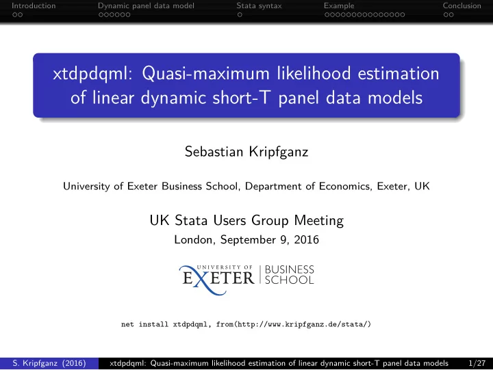
xtdpdqml: Quasi-maximum likelihood estimation of linear dynamic - PowerPoint PPT Presentation

Introduction Dynamic panel data model Stata syntax Example Conclusion xtdpdqml: Quasi-maximum likelihood estimation of linear dynamic short-T panel data models Sebastian Kripfganz University of Exeter Business School, Department of Economics, Exeter, UK UK Stata Users Group Meeting London, September 9, 2016 net install xtdpdqml, from(http://www.kripfganz.de/stata/) S. Kripfganz (2016) xtdpdqml: Quasi-maximum likelihood estimation of linear dynamic short-T panel data models 1/27

Introduction Dynamic panel data model Stata syntax Example Conclusion Estimation of short-T linear dynamic panel models in Stata Least-squares estimation of dynamic models (i.e. models with a lagged dependent variable) with random or fixed effects ( xtreg in Stata) yields biased coefficient estimates when the time horizon is short (Nickell, 1981) . Predominent estimation technique in empirical research is the generalized method of moments (GMM): Arellano and Bond (1991) “difference GMM”: xtabond , Arellano and Bover (1995) and Blundell and Bond (1998) “system GMM”: xtdpdsys . ⇒ Both Stata commands are wrappers for the more flexible command xtdpd . ⇒ Alternative user-written command with full flexibility and many additional options by Roodman (2009): xtabond2 . S. Kripfganz (2016) xtdpdqml: Quasi-maximum likelihood estimation of linear dynamic short-T panel data models 2/27

Introduction Dynamic panel data model Stata syntax Example Conclusion Estimation of short-T linear dynamic panel models in Stata Other promising approaches that can be more efficient alternatives to GMM with potentially better finite-sample performance remain underrepresented in empirical work: Bias-correction procedures by Kiviet (1995), Bun and Kiviet (2003), and Everaert and Pozzi (2007): user-written implementations xtlsdvc (Bruno, 2005) and xtbcfe (De Vos, Everaert, and Ruyssen, 2015) . Full-information maximum likelihood / structural equation modeling: xtdpdml command by Williams, Allison, and Moral-Benito (2015) as a wrapper for sem . Limited-information quasi-maximum likelihood (QML) estimation for dynamic random-effects models (Bhargava and Sargan, 1983) and dynamic fixed-effects models (Hsiao, Pesaran, and Tahmiscioglu, 2002) : new xtdpdqml package. S. Kripfganz (2016) xtdpdqml: Quasi-maximum likelihood estimation of linear dynamic short-T panel data models 3/27

Introduction Dynamic panel data model Stata syntax Example Conclusion Linear dynamic panel data model Linear panel model with first-order autoregressive dynamics: y it = λ y i , t − 1 + x ′ it β + f ′ i γ + ǫ it , ǫ it = u i + e it , t = 1 , 2 , . . . , T i (potentially unbalanced but without gaps), iid ∼ (0 , σ 2 and where e it e ). The regressors x it and f i are required to be strictly exogenous with respect to e it . The lagged dependent variable y i , t − 1 is correlated by construction with the unit-specific error component u i . Dynamic random-effects model: The time-varying regressors x it and the time-invariant regressors f i are uncorrelated with u i . Dynamic fixed-effects model: All regressors are allowed to be correlated with u i . S. Kripfganz (2016) xtdpdqml: Quasi-maximum likelihood estimation of linear dynamic short-T panel data models 4/27

Introduction Dynamic panel data model Stata syntax Example Conclusion Dynamic random-effects model y it = λ y i , t − 1 + x ′ it β + f ′ i γ + ǫ it , ǫ it = u i + e it , Random-effects assumption: iid ∼ (0 , σ 2 u i u ), uncorrelated with x it and f i . The classical random-effects estimator is a least-squares estimator treating the initial observations y i 0 as exogenous. Consequently, it is biased when T is small due to the correlation of y i , t − 1 (and therefore also y i 0 ) with u i . To account for this correlation with a likelihood approach, the joint distribution of ( y i 0 , y i 1 , . . . , y iT i ) needs to be specified. S. Kripfganz (2016) xtdpdqml: Quasi-maximum likelihood estimation of linear dynamic short-T panel data models 5/27

Introduction Dynamic panel data model Stata syntax Example Conclusion Dynamic random-effects model y it = λ y i , t − 1 + x ′ it β + f ′ i γ + ǫ it , ǫ it = u i + e it , Bhargava and Sargan (1983) propose to model the initial observations as a function of the observed exogenous variables: T ∗ � y i 0 = x ′ is π x , s + f ′ i π f + ν i 0 , s =0 with T ∗ = min( T i ), Var ( ν i 0 ) = σ 2 0 , and Cov ( ν i 0 , ǫ it ) = φσ 2 0 . Implied restrictions under stationarity of all variables: σ 2 φ = u 0 in the presence of time-varying regressors x it , (1 − λ ) σ 2 σ 2 σ 2 σ 2 1 − λ , σ 2 π f = γ 0 = (1 − λ ) 2 + 1 − λ 2 , and φ = 0 in the u e u (1 − λ ) σ 2 absence of time-varying regressors x it . S. Kripfganz (2016) xtdpdqml: Quasi-maximum likelihood estimation of linear dynamic short-T panel data models 6/27

Introduction Dynamic panel data model Stata syntax Example Conclusion Dynamic fixed-effects model y it = λ y i , t − 1 + x ′ it β + f ′ i γ + ǫ it , ǫ it = u i + e it , Fixed-effects assumption: u i allowed to be arbitrarily correlated with x it and f i . First-difference transformation to remove the fixed effects: ∆ y it = λ ∆ y i , t − 1 + ∆ x ′ it β + ∆ e it , The lagged dependent variable ∆ y i , t − 1 (and therefore also ∆ y i 1 ) is correlated by construction with the transformed error term ∆ e it . Consequently, an estimator that treats ∆ y i 1 as exogenous is biased. To account for this correlation with a likelihood approach, the joint distribution of (∆ y i 1 , ∆ y i 2 , . . . , ∆ y iT i ) needs to be specified. S. Kripfganz (2016) xtdpdqml: Quasi-maximum likelihood estimation of linear dynamic short-T panel data models 7/27

Introduction Dynamic panel data model Stata syntax Example Conclusion Dynamic fixed-effects model ∆ y it = λ ∆ y i , t − 1 + ∆ x ′ it β + ∆ e it , Hsiao, Pesaran, and Tahmiscioglu (2002) justify the following representation for the initial observations: T ∗ � ∆ y i 1 = b + ∆ x ′ is π s + ν i 1 , s =1 with T ∗ = min( T i ), Var ( ν i 1 ) = ωσ 2 e , Cov ( ν i 0 , ∆ e i 2 ) = − σ 2 e , and Cov ( ν i 0 , ∆ e it ) = 0 for t > 2. Implied restrictions under stationarity of all (first-differenced) variables: b = 0 in the presence of regressors ∆ x it , 2 b = 0 and ω = 1+ λ in the absence of regressors ∆ x it . S. Kripfganz (2016) xtdpdqml: Quasi-maximum likelihood estimation of linear dynamic short-T panel data models 8/27

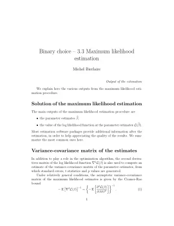
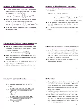
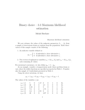
Introduction Dynamic panel data model Stata syntax Example Conclusion Quasi-maximum likelihood estimation Given the assumptions on the error components and treating all of them as if they were normally distributed, the log-likelihood function for the system of equations can be maximized with a gradient-based optimization technique. This iterative procedure needs appropriate starting values: 1 By default, xtdpdqml obtains initial estimates for the model coefficients from a consistent GMM estimator ( xtdpd ) . Initial estimates for the initial-observations coefficients are obtained from a separate least-squares estimation. The initial variance parameter estimates are computed from the respective residuals. Alternative initial estimates for the model coefficients and variance parameters can be specified by the user. Analytical first-order and second-order derivatives largely speed up the computations. 1See the paper and the online appendix at www.kripfganz.de for details. S. Kripfganz (2016) xtdpdqml: Quasi-maximum likelihood estimation of linear dynamic short-T panel data models 9/27

Introduction Dynamic panel data model Stata syntax Example Conclusion Stata syntax of the xtdpdqml command xtdpdqml depvar [ indepvars ] [ if ] [ in ] [, options ] Selected options: fe : uses the fixed-effects estimator, the default, re : uses the random-effects estimator, projection( varlist [, leads(#) nodifference omit]) : specifies the initial-observations projection, stationary : imposes restrictions valid under stationarity, vce(robust) : uses the sandwich VC estimator for valid inference under cross-sectional heteroskedasticity (Hayakawa and Pesaran, 2015) , mlparams : reports all ML parameter estimates, from( init specs ) and initval( numlist ) : specify alternative starting values, additional display options , maximize options , . . . Selected postestimation commands: predict : similar to xtreg plus equation-level scores, estat , hausman , lrtest , nlcom , suest , test , . . . S. Kripfganz (2016) xtdpdqml: Quasi-maximum likelihood estimation of linear dynamic short-T panel data models 10/27

Introduction Dynamic panel data model Stata syntax Example Conclusion Example Estimation of an employment equation for 140 UK companies, 1976–1984, based on the Arellano and Bond (1991) data set: . webuse abdata Dependent variable: Logarithm of the number of employees ( n ). Strictly exogenous explanatory variables: Real wage ( w ), Gross capital stock ( k ), Time dummies ( yr1978-yr1984 ). S. Kripfganz (2016) xtdpdqml: Quasi-maximum likelihood estimation of linear dynamic short-T panel data models 11/27