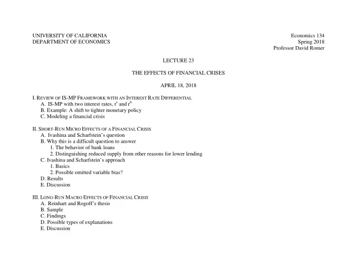

UNIVERSITY OF CALIFORNIA Economics 134 DEPARTMENT OF ECONOMICS Spring 2018 Professor David Romer LECTURE 23 THE EFFECTS OF FINANCIAL CRISES APRIL 18, 2018 I. R EVIEW OF IS-MP F RAMEWORK WITH AN I NTEREST R ATE D IFFERENTIAL A. IS-MP with two interest rates, r s and r b B. Example: A shift to tighter monetary policy C. Modeling a financial crisis II. S HORT -R UN M ICRO E FFECTS OF A F INANCIAL C RISIS A. Ivashina and Scharfstein’s question B. Why this is a difficult question to answer 1. The behavior of bank loans 2. Distinguishing reduced supply from other reasons for lower lending C. Ivashina and Scharfstein’s approach 1. Basics 2. Possible omitted variable bias? D. Results E. Discussion III. L ONG -R UN M ACRO E FFECTS OF F INANCIAL C RISIS A. Reinhart and Rogoff’s thesis B. Sample C. Findings D. Possible types of explanations E. Discussion
Economics 134 David Romer Spring 2018 L ECTURE 23 The Effects of Financial Crises April 18, 2018
Announcements • Problem Set 4: • Due at the beginning of lecture next time (April 23). • Optional problem set work session: Thursday, April 19, 5–7, in 597 Evans Hall. • We will have a guest lecture next time.
Final Exam – Basics • Mechanics: • Monday, May 7, 3–6 P.M. • Students with DSP accommodations: You will receive an email from me. • Coverage: Whole semester. But: • There will be more emphasis on the material after the midterm. • There won’t be any multiple choice questions that are specifically about the readings from before the midterm.
Final Exam – Types of Questions • Broadly similar to the midterm: • Multiple choice • Short answers • Problems • Essay (or essays)
Final Exam – Places to Get Help • Q&A/Review session: Wednesday, May 2, 4–6 P.M., 10 Evans. • My office hours in RRR week: Thursday, May 3, 1–3 P.M. • GSI office hours. • And remember that there is a set of sample exam questions on the course website.
I. R EVIEW OF IS-MP M ODEL WITH A C REDIT S PREAD
Expanding the IS-MP Model • 2 real interest rates: • The saving or safe real interest rate, r s . • The borrowing or risky real interest rate, r b . • The MP and IS curves depend on different rates. • The difference between the two rates, r b − r s , depends on Y: r b − r s = d(Y). D(Y) is positive, and a decreasing function of Y.
The MP curve depends on r s : r s = r s (Y, π ) r s MP Y MP curve in (Y,r s ) space looks the same as before.
The IS curve depends on r b ; r s = r b − (r b − r s ) r b − r s = d(Y) r s IS in terms of r b (or without spread) d(Y) IS in terms of r s (or with spread) Y Accounting for the spread makes IS lower and flatter than before.
Example: A Shift to Tighter Monetary Policy MP 1 r s MP 0 IS (no differential) IS (with differential) Y
A Shift to Tighter Monetary Policy • r s rises and Y falls. • Can we determine what happens to r b ? • r s and d(Y) both rise, so r b must rise. • Can we determine how the fall in Y in the extended model compares with the fall in the model with no interest rate differential? • The IS curve is flatter, so the fall in Y is greater. • (This is another example of the “financial accelerator.”)
A financial crisis increases r b − r s at a given Y. (That is, it is an upward shift of the d(Y) function.) r s MP 0 r s 0 IS 0 Y Y 0
A financial crisis increases r b − r s at a given Y. IS shifts down. r s MP 0 r s 0 r s 1 IS 0 IS 1 Y 1 Y Y 0 r s and Y both fall.
Financial Crisis with Zero Lower Bound r s MP 0 r s 0 0- π e IS 0 IS 1 Y Y 1 Y 0 If crisis makes the economy hit the zero bound, r s can’t fall as much and Y falls more.
II. S HORT -R UN M ICRO E FFECTS OF A FINANCIAL C RISIS (I VASHINA AND S CHARFSTEIN P APER )
Ivashina and Scharfstein’s Question • Did the bankruptcy of Lehman reduce the availability of credit?
Commercial and Industrial Bank Credit Outstanding Went Way Up Following the Lehman Bankruptcy
Commercial and Industrial Bank Credit Outstanding Went Way Up Following the Lehman Bankruptcy • Does this indicate that limited credit supply was not a problem after the Lehman bankruptcy? • What is Ivashina and Scharfstein’s explanation for the rise in loans? • They argue that the rise was the result of firms drawing on existing lines of credit.
What Is Ivashina and Scharfstein Evidence for Their Proposed Explanation? • New lending appears to have fallen sharply. • Annual data show a large fall in unused credit lines as a percentage of total credit lines in 2008. • Survey data show very large credit line drawdowns in one week in November. • There were numerous media reports of firms drawing on their credit lines in the 3 months after mid-August 2008 (and virtually none in the 3 months before).
Recall Ivashina and Scharfstein’s Question: Did the bankruptcy of Lehman reduce the availability of credit? • Why wouldn’t it be persuasive to just look at whether lending fell? • As we’ve just discussed, credit lines complicate the interpretation of data on lending! • More fundamentally, a fall in lending could reflect a decline in credit demand rather than in credit supply.
Recall Ivashina and Scharfstein’s Question: Did the bankruptcy of Lehman reduce the availability of credit? • Suppose we saw that the quantity of lending fell and that credit terms became more onerous (for example, increases in interest rates). Would that be persuasive? • It could reflect a decline in borrower quality (for example, greater riskiness) rather than reduced credit supply to a borrower of a given quality.
How Do Ivashina and Scharfstein Address Their Question? • They look at cross-section evidence: especially, variation across banks. • They argue that two variables potentially affected a bank’s credit supply: • Fraction of the bank’s funding that was from “wholesale” sources rather than retail deposits. • Amount of the bank’s lending that was “cosyndicated” with Lehman.
Might There Be Omitted Variable Bias? • Consider the regression ∆Lending i = a + bWholesale i +e i , where i indexes banks, ∆Lending is the percent change in a bank’s lending, and Wholesale is the fraction of its deposits from wholesale sources. • Ivashina and Scharfstein’s big concern: Maybe the firms that borrowed from banks that relied more on wholesale funding differed systematically from the firms that borrowed from banks that relied less on wholesale funding.
What Is Ivashina and Scharfstein Argument That There Is Not Major Omitted Variable Bias? • Mainly: On dimensions we can observe, the firms that borrowed from banks that relied more on wholesale funding look pretty similar to the firms that borrowed from banks that relied less on wholesale funding.
Results: Retail Funding Note: “Pre-crisis” is 8/06-7/07; “Crisis I” is 8/07-7/08 ; “Crisis II” is 8/08-12/08.
Interpreting the Economic Magnitude of the Point Estimates—Example • The estimate of 0.56 in Column (3). • “The average bank experiences a 34% drop in the number of lead syndications; however, the estimated coefficients imply that banks with deposits one standard deviation above the mean experience a 14% drop, while banks one standard deviation below the mean experience a 51% drop.”
Results: Retail Funding and Lehman Cosyndication Note: “Pre-crisis” is 8/06-7/07; “Crisis I” is 8/07-7/08 ; “Crisis II” is 8/08-12/08.
Difficulties in Going from the Micro Estimates to Macro Implications • A reduction in credit supply by some banks doesn’t necessarily imply that there was reduced credit supply to some firms—for example, perhaps borrowers can switch easily across banks. • Even some firms having trouble getting credit doesn’t necessarily imply effects on macro outcomes—for, maybe customers can switch easily across firms.
III. L ONG -R UN M ACRO E FFECTS OF A FINANCIAL C RISIS (R EINHART AND R OGOFF R EADING )
Reinhart and Rogoff’s Thesis • The aftermaths of major financial crises are awful and long-lasting.
Reinhart and Rogoff’s Sample • 21 major banking crises. • 6 current; 13 other postwar (5 in advanced countries, 8 in developing); 2 others (Norway 1899, U.S. 1929).
Falls in Real House Prices
Falls in Real Equity Prices
Rises in Unemployment Rates
Falls in Real GDP per Capita
Time for Real GDP per Capita to Return to Pre-Crisis Level
Increase in Real Government Debt
Possible Categories of Explanations • Long-lasting effect on the level and/or growth rate of potential output. • Long-lasting effect on aggregate demand. • It’s not a causal effect of the crisis: the economy was operating well above its normal capacity (potential output). The poor economic performance is just the return to normal. • Maybe it’s not a fact at all: How do R&R identify the crises?
Recommend
More recommend