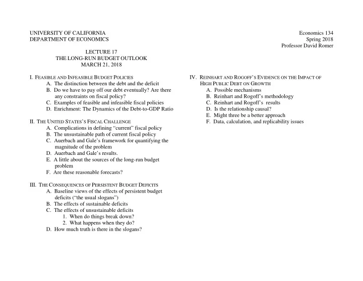

UNIVERSITY OF CALIFORNIA Economics 134 DEPARTMENT OF ECONOMICS Spring 2018 Professor David Romer LECTURE 17 THE LONG-RUN BUDGET OUTLOOK MARCH 21, 2018 I. F EASIBLE AND I NFEASIBLE B UDGET P OLICIES IV. R EINHART AND R OGOFF ’ S E VIDENCE ON THE I MPACT OF A. The distinction between the debt and the deficit H IGH P UBLIC D EBT ON G ROWTH B. Do we have to pay off our debt eventually? Are there A. Possible mechanisms any constraints on fiscal policy? B. Reinhart and Rogoff’s methodology C. Examples of feasible and infeasible fiscal policies C. Reinhart and Rogoff’s results D. Enrichment: The Dynamics of the Debt-to-GDP Ratio D. Is the relationship causal? E. Might three be a better approach II. T HE U NITED S TATES ’ S F ISCAL C HALLENGE F. Data, calculation, and replicability issues A. Complications in defining “current” fiscal policy B. The unsustainable path of current fiscal policy C. Auerbach and Gale’s framework for quantifying the magnitude of the problem D. Auerbach and Gale’s results. E. A little about the sources of the long-run budget problem F. Are these reasonable forecasts? III. T HE C ONSEQUENCES OF P ERSISTENT B UDGET D EFICITS A. Baseline views of the effects of persistent budget deficits (“the usual slogans”) B. The effects of sustainable deficits C. The effects of unsustainable deficits 1. When do things break down? 2. What happens when they do? D. How much truth is there in the slogans?
Economics 134 David Romer Spring 2018 L ECTURE 17 T HE L ONG -R UN BUDGET O UTLOOK March 21, 2018
Announcement • Problem Set 3 is being distributed. • It is due at the beginning of lecture on Wednesday, April 4. • Optional problem set work session: Monday, April 2, 6:45–8:15, in 597 Evans Hall.
I. F EASIBLE AND I NFEASIBLE B UDGET P OLICIES
Basic Concepts: The Debt and the Deficit • Debt: The total amount the government owes (currently about $15 trillion, excluding amounts owed by one part of the government to another). • Deficit: The difference between expenditures and revenues over some period – that is, the amount the government borrows over some period (about $600 billion in the 2018 fiscal year). • The link between the deficit and the debt: The deficit is the change in the debt. • Thus, the amount of government debt will rise by about $600 billion in the 2018 fiscal year.
Issue: What Fiscal Policies Are Feasible? • Do we have to pay off the debt at some point? • Are there any limits on the government’s ability to issue debt?
What Fiscal Policies Are Feasible? • Let b denote the ratio of government debt to annual GDP (currently about 77%). • Two assumptions about b that are very reasonable: 1. There is some upper limit to b – at some point, the amount of government debt would be so large relative to incomes that people would be unable or unwilling to hold it. 2. For a low enough value of b (for example, b = 20%): If b were at that level and there was no doubt that it would remain at that level, people would be willing to hold the debt.
What Fiscal Policies Are Feasible? (cont.) • b ≡ Debt/GDP. • GDP is normally growing (from both real output growth and inflation). • So if the debt is constant (that is, if there are no deficits), b will be getting smaller and smaller. • Implications: o We do not have to pay off the debt. o In fact, we can run deficits forever. • But: There are limits.
A Useful Fact • If the deficit-to-GDP ratio and the growth rate of GDP are each constant, then the debt-to-GDP ratio will not fall or grow without bound, but will stabilize at some level. • The level it will stabilize at is given by:
What Fiscal Policies Are Feasible? (cont.) • Two assumptions that provide a useful benchmark for thinking about feasible and infeasible policies: 1. There is some maximum level of b, b MAX , that people are willing to hold. 2. The growth rate of nominal GDP is steady at some level.
Examples of Feasible + Infeasible Fiscal Policies • #1 The deficit-to-GDP ratio is steady, but at a level that implies that b will stabilize at some very high level (above b MAX ). INFEASIBLE • #2 The deficit-to-GDP ratio is steady at a positive level that implies that b will stabilize at some low level (below b MAX ). FEASIBLE #3 The deficit-to-GDP ratio is at a level that, if • maintained, implies that b would stabilize at a very high level (above b MAX ). But, before b rises very much, the deficit-to-GDP ratio falls permanently to a level that implies that b will stabilize at some low level (below b MAX ). FEASIBLE • #4 The deficit-to-GDP ratio is growing without INFEASIBLE bound.
The Debt-to-GDP Ratio, 1940-2005 120.0 100.0 80.0 Percent 60.0 40.0 20.0 0.0 1940 1950 1960 1970 1980 1990 2000
Enrichment: The Dynamics of the Debt-to-GDP Ratio • Let B(t) be the amount of debt, Y(t) nominal GDP, and Deficit(t) the deficit. (Thus, by definition, Deficit(t) = dB(t)/dt.) • Define: Debt-to- GDP ratio: b(t) = B(t)/Y(t). • • Deficit-to- GDP ratio: d(t) = Deficit(t)/Y(t). • Growth rate of nominal GDP: g Y (t)=[dY(t )/dt]/Y(t).
The Dynamics of the Debt-to-GDP Ratio (cont.) • Debt-to- GDP ratio: b(t) = B(t)/Y(t). • Deficit-to- GDP ratio: d(t) = Deficit(t)/Y(t). • Growth rate of nominal GDP: g Y (t) = [dY(t)/dt]/Y(t). • The dynamics of b: db(t) = dB(t)/dt − B t dY t 2 dt Y(t) Y t d t = Deficit(t) − B(t) dY(t)/dt Y(t) Y(t) Y(t) = d t − b t g Y t .
The Dynamics of the Debt-to-GDP Ratio (cont.) • If d(t) (the deficit as a share of GDP) and g Y (t) (the growth rate of nominal GDP are constant: db(t) = � d − g Y b t . dt db(t) dt � d 0 � b(t) d/g Y So: Regardless of where it starts, b converges to • � d/g Y .
II. T HE U NITED S TATES ’ S F ISCAL C HALLENGE
Complications in Defining “Current Policy” • Using current law is not reasonable, so we have to use some judgment. • Policies are changing. • There is a lot of disagreement about the likely path of government health care spending.
Auerbach and Gale’s “Extended Policy” Scenario • Discretionary spending is roughly constant in real terms for the next decade, then roughly constant as a share of GDP. • Tax increases that are nominally scheduled to go into effect do not. • 3 different possibilities for path of government health care spending: optimistic (Medicare trustees); pessimistic (CBO); intermediate (Medicare actuary). • Their analysis predates recent budget changes (tax bill and budget deal).
Source: Congressional Budget Office (March 2017).
Source: Congressional Budget Office (March 2017).
Auerbach and Gale’s Question (for Quantifying the Size of Our Long-Run Fiscal Problem) • Starting from “current policy,” suppose we enacted spending cuts and/or revenue increases that subtracted a constant fraction of GDP each year from the deficit excluding interest payments from what it would be under current policy. • What constant fraction of GDP would we have to reduce the noninterest deficit by so that in the long run, the debt-to-GDP ratio would stabilize at its current level?
Auerbach and Gale’s Answer • What constant fraction of GDP would we have to reduce the noninterest deficit by so that in the long run, the debt-to-GDP ratio would stabilize at its current level? o If growth of health care spending is low: About 5.5%. o If it is intermediate: About 7.7%. o If it is high: About 9.6%. • For comparison: o Total Federal noninterest spending is about 19% of GDP. o Personal income tax revenues are about 9% of GDP. o Defense spending is about 4% of GDP. • And: This leaves out the recent tax bill and budget deal.
A Little about the Sources of the Long-Run Budget Problem
Should We Take These Projections Seriously? There is substantial uncertainty. • But the fact that there is substantial uncertainty • means that things could turn out quite a bit better than these projections suggest, or that they could turn out quite a bit worse. So uncertainty is not a reason for lack of concern. If anything, it is an argument for greater concern. In some key aspects, the projections, dire as they • are, look overly optimistic.
III. T HE C ONSEQUENCES OF P ERSISTENT B UDGET D EFICITS
The Effects of Persistent Budget Deficits – Rounding Up the Usual Suspects “We are mortgaging our children’s future.” • “The United States is headed for Chapter 11.” • “But we mainly owe it to ourselves.” • “We should save our ammo until we need it.” •
The Effects of Sustainable Persistent Budget Deficits Budget deficits lower national saving, and so cause • future standards of living to be lower than they would otherwise be. This is true regardless of whether the debt is held • by Americans or foreigners.
Unsustainable Persistent Budget Deficits Stein’s law: “If something cannot go on forever, it • will stop.”
Recommend
More recommend