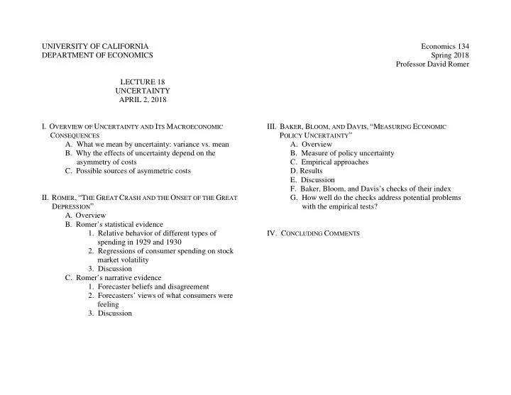
UNIVERSITY OF CALIFORNIA Economics 134 DEPARTMENT OF ECONOMICS - PowerPoint PPT Presentation
UNIVERSITY OF CALIFORNIA Economics 134 DEPARTMENT OF ECONOMICS Spring 2018 Professor David Romer LECTURE 18 UNCERTAINTY APRIL 2, 2018 I. O VERVIEW OF U NCERTAINTY AND I TS M ACROECONOMIC III. B AKER , B LOOM , AND D AVIS , M EASURING E
UNIVERSITY OF CALIFORNIA Economics 134 DEPARTMENT OF ECONOMICS Spring 2018 Professor David Romer LECTURE 18 UNCERTAINTY APRIL 2, 2018 I. O VERVIEW OF U NCERTAINTY AND I TS M ACROECONOMIC III. B AKER , B LOOM , AND D AVIS , “M EASURING E CONOMIC C ONSEQUENCES P OLICY U NCERTAINTY ” A. What we mean by uncertainty: variance vs. mean A. Overview B. Why the effects of uncertainty depend on the B. Measure of policy uncertainty asymmetry of costs C. Empirical approaches C. Possible sources of asymmetric costs D. Results E. Discussion F. Baker, Bloom, and Davis’s checks of their index II. R OMER , “T HE G REAT C RASH AND THE O NSET OF THE G REAT G. How well do the checks address potential problems D EPRESSION ” with the empirical tests? A. Overview B. Romer’s statistical evidence 1. Relative behavior of different types of IV. C ONCLUDING C OMMENTS spending in 1929 and 1930 2. Regressions of consumer spending on stock market volatility 3. Discussion C. Romer’s narrative evidence 1. Forecaster beliefs and disagreement 2. Forecasters’ views of what consumers were feeling 3. Discussion
Economics 134 David Romer Spring 2018 L ECTURE 18 U NCERTAINTY April 2, 2018
Announcements • Problem Set 3: • Due at the beginning of lecture next time (April 4). • Optional problem set work session: Today (April 2), 6:45–8:15, in 597 Evans Hall. • Paper: • Due two weeks from today (April 16). • A document with a few comments on writing the essay is now on the course website.
Announcements • Reminder: I’d still like each of you to set a goal of speaking in lecture at least once this semester!
I. O VERVIEW
Role of Uncertainty • What is uncertainty and what causes it? • How can we measure uncertainty? • What are the macroeconomic impacts of an increase in uncertainty?
What Do Economists Mean by Uncertainty? • It involves variances rather than means. • The mean of some indicator tells you about its level. • The variance tells you about its range. Uncertainty is related to the variance of possible outcomes. • We will focus on changes in uncertainty. • Means and variances may move together.
Types of Uncertainty • Uncertainty about the state of the economy. Typically this is uncertainty about aggregate demand. • Uncertainty about technology. This is uncertainty about what we will be producing and how. • Uncertainty about policy. What will the government be doing and why? Involves taxing and spending decisions, regulations, and monetary policy.
A Simple Example of How Uncertainty Might Affect Spending • You’re deciding how many champagne glasses to rent for your child’s wedding reception. • There’s a 50% chance that 100 guests will show up, and a 50% chance that 120 will show up. • If there are fewer glasses than guests, some guests will not be able to toast the newlyweds. • It costs a dollar to rent each glass. • How many glasses would you rent?
Messages from this Example • Uncertainty does not necessarily reduce spending. • What is key is the asymmetry of costs of doing more or less than you would have done had you known for sure.
Sources of Asymmetric Costs (1): An Asymmetric Objective Function • 1. Recall the champagne glass example. • 2. A simple 2-period consumption example: o Your income will either rise by 20% or fall by 20% (50-50 chance). o In the absence of this uncertainty (so that your income would be unchanged for sure), you would just consume your current income today. o Do you think the uncertainty will make you consume more or less today than your income?
Sources of Asymmetric Costs (2): Irreversibility and the Resolution of Uncertainty • Consider the rental shop deciding how many champagne glasses to buy. • Champagne glasses can’t be returned, and there isn’t a good resale market for them. • The shop will learn in a month either that all future weddings will have 100 guests or that they all will have 120 guests (50-50 chance). How many glasses do you think the shop will buy?
Sources of Asymmetric Costs (3): Irreversibility, the Resolution of Uncertainty, and Choice of the Type of Spending • Consider our rental shop. • The shop will learn in a month whether short, inexpensive or tall, expensive champagne glasses will be fashionable for the next decade. How many glasses do you think the shop will buy now? • This is wait-and-see uncertainty.
Macro Impact of Uncertainty • Greater uncertainty about the state of the economy will tend to depress consumer spending. Consumers especially want to avoid very low consumption. If income is more variable, they need to save more to insure against the risk of very low income. For standard theories and estimates of consumer behavior, this effect would tend to be modest.
Macro Impact of Uncertainty • Effects of income or other types of uncertainty may be much larger if there are large costs of changing consumption or investment decisions. Suppose consumption or investment decisions are irreversible. And that there is uncertainty that is expected to be resolved at some point. Can lead to “wait and see” behavior. Could get a very large, short-run decline in spending.
II. R OMER , “T HE G REAT C RASH AND THE O NSET OF THE G REAT D EPRESSION ”
Monthly S&P Stock Price Index 11.5 16.5 21.5 26.5 31.5 36.5 1.5 6.5 Jan 1922 Jul 1922 Stock Prices, 1922:1-1930:12 Jan 1923 Jul 1923 Jan 1924 Jul 1924 Jan 1925 Jul 1925 Jan 1926 Jul 1926 Jan 1927 Jul 1927 Jan 1928 Jul 1928 Jan 1929 Jul 1929 Jan 1930 Jul 1930
Industrial Production (Logarithms) 1.2 1.4 1.6 1.8 2.2 2.4 1 2 1929-01 Industrial Production, 1929-1933 1929-04 August 1929 1929-07 1929-10 1930-01 October 1929 1930-04 1930-07 1930-10 October 1930 1931-01 1931-04 1931-07 1931-10 1932-01 1932-04 1932-07 1932-10 1933-01 1933-04 1933-07 1933-10
What Is Romer’s Hypothesis about Why Consumption Fell So Sharply in Late 1929 and Early 1930? • The crash of the stock market in October 1929 and the subsequent gyrations of the market generated substantial uncertainty that consumers thought would be resolved quickly. • This created a large value to waiting, which led consumers to postpone purchases of durable goods.
What Is Romer’s Argument about Why Uncertainty Led Consumers to Postpone Purchases of Durables, Rather than Just Spend Less on Durables? • Consumers had to decide not just the amount of durables to buy, but their quality. • Desired quality depends on your future income. • Creates a value to waiting.
What Evidence Does Romer Consider? • Statistical: o Behavior of different types of consumption following the crash. o Relationship between stock price volatility and consumption. • Narrative: o Forecasters’ uncertainty. o Forecasters’ assessments of the public’s uncertainty. o Contrast with other recessions in the 1920s.
Behavior of Different Types of Consumer Spending
Relationship between Consumer Spending and Stock Price Volatility
Impact of volatility (the d i coefficient) is more negative for durables than for nondurables, as the hypothesis predicts.
Discussion
Narrative Evidence • Use professional forecasters as a proxy for other people in the economy. Are they more uncertain? • Read their assessment of consumers’ and firms’ behavior. • Compare their assessments in 1929–1930 with other recessions in the 1920s.
Narrative Evidence on Forecaster Uncertainty • “Among the five forecasters, four became definitely more uncertain about the future of business immediately following the collapse of stock prices in late October 1929. Moreover, the forecasters who became less confident indicated that it was because of the stock market crash.” (p. 612) • Example: “’[T]he unprecedented declines in stock prices ... make it difficult to estimate at present the amount of injury which will be done to business …. [A] month hence it may be possible to appraise the situation more satisfactorily and present a definite forecast for the year 1930.’” (p. 612)
Narrative Evidence about Consumer Behavior • “After the crash every one of the forecasters stressed that consumers were very uncertain about the future of the economy.” (p. 616) • Example: “Moody’s … discussed ‘the stock market break, which undermined general confidence’ and indicated that ‘during the past few weeks almost everybody held his plans in abeyance and waited for the horizon to clear.’” (p. 616)
Narrative Evidence Comparing with the Recessions of 1920–1921 and 1923–1924 • “In these earlier downturns there was never a time when several of the forecasters simultaneously ex- pressed greater uncertainty. Furthermore, many of the forecasters were equally confident throughout both 1921 and 1924.” (p. 614) • Example: “[The Harvard Economic Society’s Weekly Letters ] stated with surety in February 1924 that ‘conditions thus remain favorable to the maintenance of generally good business conditions’.” (p. 614)
Discussion
III. B AKER , B LOOM , AND D AVIS , “M EASURING E CONOMIC P OLICY U NCERTAINTY ”
Recommend
More recommend
Explore More Topics
Stay informed with curated content and fresh updates.
