UNIVERSITY OF CALIFORNIA Economics 134 DEPARTMENT OF ECONOMICS - - PDF document

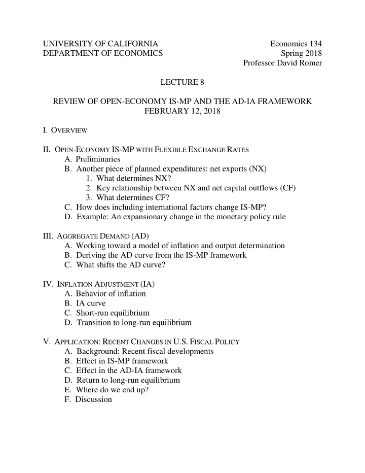
UNIVERSITY OF CALIFORNIA Economics 134 DEPARTMENT OF ECONOMICS Spring 2018 Professor David Romer LECTURE 8 REVIEW OF OPEN-ECONOMY IS-MP AND THE AD-IA FRAMEWORK FEBRUARY 12, 2018

• I. OVERVIEW
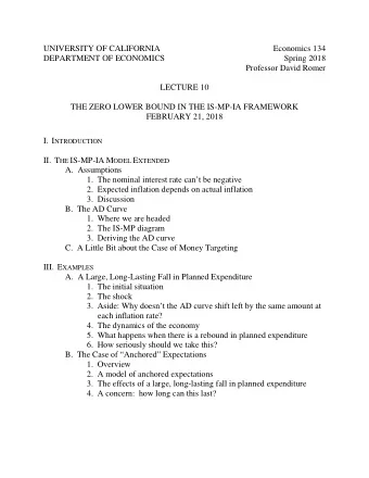
• II. OPEN-ECONOMY IS-MP WITH FLEXIBLE EXCHANGE RATES
• A. Preliminaries
• B. Another piece of planned expenditures: net exports (NX)
• 1. What determines NX?
• 2. Key relationship between NX and net capital outflows (CF)
• 3. What determines CF?
• C. How does including international factors change IS-MP?
• D. Example: An expansionary change in the monetary policy rule
• III. AGGREGATE DEMAND (AD)
• A. Working toward a model of inflation and output determination
• B. Deriving the AD curve from the IS-MP framework
• C. What shifts the AD curve?
• IV. INFLATION ADJUSTMENT (IA)
• A. Behavior of inflation
• B. IA curve
• C. Short-run equilibrium
• D. Transition to long-run equilibrium
• V. APPLICATION: RECENT CHANGES IN U.S. FISCAL POLICY
• A. Background: Recent fiscal developments
• B. Effect in IS-MP framework
• C. Effect in the AD-IA framework
• D. Return to long-run equilibrium
• E. Where do we end up?
• F. Discussion

LECTURE 8 Review of Open Economy IS-MP and the AD-IA Framework

February 12, 2018

Economics 134 David Romer Spring 2018

Announcements

• An answer sheet to Problem Set 1 has been

posted on the course website. You should study it carefully.

• The start of lecture on Wednesday will be set

aside for you to fill out an “Early Feedback” form.

• I would like each of you to set a goal of

speaking in lecture at least once this semester.

LECTURE 7 Monetary Factors in the Great Depression (concluded)

Economics 134 David Romer Spring 2018

• 0. EXPECTED INFLATION IN THE IS-LM MODEL

(REVISITED)

Real versus Nominal Interest Rates

i ≡ r + πe

• i is the nominal rate
• r is the real rate
• πe is expected inflation

r ≡ i - πe

How Expected Inflation Affects the IS-LM Diagram

• As we have discussed, we can use the money

market diagram to find the nominal interest rate that causes money demand and money supply to be equal for a given Y.

• r ≡ i - πe.
• So, the real interest rate that causes money

demand and money supply to be equal for a given Y is the nominal rate that we find using the money market diagram minus expected inflation.

Expected Inflation in IS-LM Y r LM0 IS0 r0 Y0 LM (in terms of i and Y) πe

We subtract off πe from each point on the LM curve in terms

• f i and Y to get the LM curve in terms of r and Y.

Fall in Expected Inflation in IS-LM Y r

LM0 (π0

𝑓)

IS0 r0 Y0

LM1 (π1

𝑓)

π1

𝑓 < π0 𝑓

LM curve shifts up by the fall in πe. π0

𝑓 - π1 𝑓

Y1 r1

Effect of a Fall in Expected Inflation in IS-LM

• A fall in πe shifts the LM curve (in terms of r

and Y) up.

• The LM curve shifts up by the fall in πe

(π0

𝑓 – π1 𝑓).

• r rises and Y falls.

What happens to i when there is a fall in expected inflation?

• i ≡ r + πe
• r rises, which tends to increase i.
• πe falls, which tends to decrease i.
• r rises by less than πe falls, so i falls.
• A fall in expected inflation (to expected

deflation) can help explain why real rates rose and nominal rates fell in the early 1930s.

The Impact of a Fall in Expected Inflation on i Y r

LM0 (π0

𝑓)

IS0 r0 Y0

LM1 (π1

𝑓)

π1

𝑓 < π0 𝑓

The rise in r (the distance from r0 to r1) is less than the fall in πe (the distance from LM0 to LM1).

π0

𝑓 - π1 𝑓

Y1 r1 r0 - r1

Another Way to See that i Falls: Incorporate the Fact from the IS-LM Diagram that Y Falls into the Money Market Diagram

M/P i M /P L(i,Y1) i1 L(i,Y0) i0

Y1 < Y0

There was a large fall in expected inflation in 1930 and 1931.

Source: Stephen Cecchetti, American Economic Review, March 1992.

Narrative Evidence from Business Week

• Expected deflation after mid-1930.
• Monetary developments and Fed policy were

a key source of expectations of deflation.

• “Our idle gold hoard piles up without

increasing the means of payment by credit expansion because of paralysis of banking policy, thus prolonging price deflation” (4/29/31, cover).

• 00. OCTOBER 1931

(NOTE: SLIDES ON OCT. 1931 ARE IN THE LECTURE 7 SLIDES)

LECTURE 8 Review of Open Economy IS-MP and the AD-IA Framework

Economics 134 David Romer Spring 2018

• I. OVERVIEW OF WHERE WE ARE HEADED

IS-LM Useful for the Great Depression

• Key story of the Depression is a collapse in

aggregate demand.

• IS-LM useful for understanding the sources of

the decline in demand.

• International factors present, but not

essential.

• Likewise, inflation adjustment present, but

swamped by the collapse in demand.

Need a Richer Model for the Postwar Era

• Useful to incorporate international trade and

flexible exchange rates.

• Need a framework that includes inflation

adjustment.

• II. OPEN-ECONOMY IS-MP WITH FLEXIBLE

EXCHANGE RATES

Preliminaries

• Working with IS-MP because we are focusing
• n the postwar period.
• Fed has been conducting policy in terms of

the interest rate for most of this period, so MP is appropriate.

• Only doing the case of flexible exchange rates.

Real Exchange Rate (ε)

• Number of units of foreign goods we can obtain by

buying 1 less unit of domestic goods.

• For ε between the dollar and some foreign currency,

a rise in ε is a real appreciation of the dollar.

• Note: We can write ε as eP/P*, where e is the

number of units of foreign currency we can get with 1 unit of domestic currency (so e is the nominal exchange rate), P is the price of domestic goods in terms of domestic currency, and P* is the price of foreign goods in terms of foreign currency. However, we will generally work directly with ε.)

Planned Expenditures

• E = C(Y-T) + I(r) + G + NX
• NX (Net Exports) is Exports - Imports
• Proximate determinant of net exports is the

real exchange rate: NX = NX(ε)

• Relationship is negative: A rise in ε lowers NX.

Key Relationship between NX and CF

• Quantity of dollars supplied in foreign currency

market must equal the quantity demanded

• Supply of Dollars: Imports (M) + Capital Outflows

(CO)

• Demand for Dollars: Exports (X) + Capital Inflows

(CI)

• M + CO = X + CI
• CO – CI = X – M
• Net Capital Outflow (CF) = Net Exports (NX)

What Determines CF?

• The real interest rate in U.S.
• CF = CF(r)
• Relationship is negative.
• A higher r in U.S. reduces CF.

A Helpful Substitution

• E = C(Y-T) + I(r) + G + NX(ε)
• Since CF(r) = NX(ε), we can write instead:

E= C(Y-T) + I(r) + G + CF(r)

• Now two pieces of planned expenditures

depend negatively on r.

A Rise in the Interest Rate in the Closed Economy Keynesian Cross Y E

E = Y E = C(Y–T) + I(r0) + G Y0 Y1 E = C(Y–T) + I(r1) + G E shifts down for only one reason: I = I(r). r1>r0

A Rise in the Interest Rate in the Open Economy Keynesian Cross Y E

E = Y E = C(Y–T) + I(r0) + G + CF(r0) Y0 Y1 E = C(Y–T) + I(r1) + G + CF(r1) E shifts down for two reasons: I = I(r) and CF = CF(r). r1>r0

Closed-Economy vs. Open-Economy IS Y r MP ISClosed ISOpen

Open-economy IS is flatter because spending is more sensitive to r. Question: What is happening to ε as we move down along ISOpen?

Expansionary Change in MP Rule in an Open Economy

Monetary policy changes have more impact in an open economy. Y0

Y r MP0 ISClosed r0 ISOpen MP1

Y1 (Closed) Y1(Open)

What happens to the real exchange rate in response to the shift in MP?

• r fell, so CF(r) rises.
• CF = NX, so NX must rise as well.
• What makes NX rise? The real exchange rate

falls.

• The dollar depreciates.

• III. AGGREGATE DEMAND

Where we are headed: AD-IA Y π IA AD π0 Y0

Impact of Inflation in IS-MP

• No impact on IS curve
• MP curve shows Fed’s policy rule for the real

interest rate.

• r = r(Y,π), where π is inflation.
• r(Y, π) is an increasing function of both

arguments.

• Since we draw r = r(Y), a change in π shifts the

MP curve.

π is a shift variable for the MP Curve in (Y,r) space

π1 > π0 Y r MP0 (π0) MP1 (π1)

Derivation of the Aggregate Demand (AD) Curve AD π0 Y0 Y π Y r IS0 MP0 (π0) MP1 (π1) π1 Y0 Y1 Y1

What Shifts the AD Curve?

• Anything other than inflation that shifts the IS
• r MP curves.
• A change in government spending (G) or taxes

(T).

• Change in animal spirits.
• A change in Federal Reserve tastes.

• IV. INFLATION ADJUSTMENT

Key Assumptions about Inflation Behavior

• At a point in time, inflation is given.
• When Y > Y, inflation gradually rises.
• When Y < Y, inflation gradually falls.
• When Y = Y, inflation is constant.
• Note: Y is normal or potential output – the

level of output that prevails when prices are fully flexible.

Inflation fell less in the Great Recession and the (subsequent period

• f continued high unemployment) than in previous recessions.

Two Important Points

• Inflation does not respond immediately to

deviations of output from potential.

• We are talking about inflation, not prices.

Output below potential causes the rate of inflation to fall from one positive number to a smaller positive number.

Inflation Adjustment Curve (IA) Y π π0 IA

Short-Run Equilibrium Y π IA0 AD0 π0 Y0

AD/IA Intersect below Y IA will shift down. Y π IA0 AD0 π0 Y0 Y IALR πLR

AD/IA Intersect above Y Y π IA0 AD0 π0 Y0 Y IALR πLR IA will shift up.

AD/IA Intersect at Y Y π IA0 AD0 π0 Y0 Y Long-Run Equilibrium

Long-Run Equilibrium r Y π Y r rLR Y MP IS IA AD πLR Y

• V. APPLICATION: RECENT CHANGES IN U.S. FISCAL

POLICY

Recent U.S. Fiscal Developments

• Since last June, the projected deficit for fiscal

year 2019 has risen from $700 billion (3% of GDP) to $1.2 trillion (6% of GDP).

• The change is entirely the result of changes in

policy, not in the health of the economy: roughly $300 billion from the tax bill, and roughly $200 billion from the budget agreement.

• Most observers think that output is currently

very close to potential (𝑍 ≈ 𝑍 ).

A Decrease in T and an Increase in G Y π Y r IA0 π0 Y IS0 AD0 MP0 r0 Y

Impact of a Decrease in T and an Increase in G

What Happens to the Real Exchange Rate (ε)?

What Other Disadvantages Might There Be to the Fiscal Developments?

What Advantages Might There Be to the Fiscal Developments?