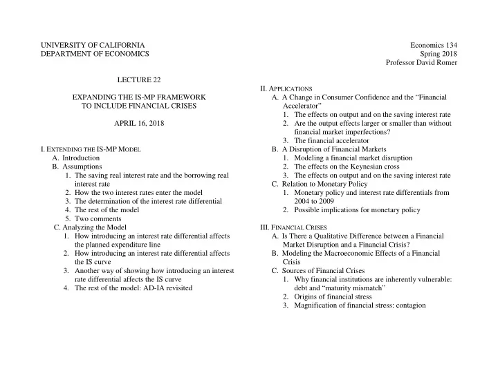

UNIVERSITY OF CALIFORNIA Economics 134 DEPARTMENT OF ECONOMICS Spring 2018 Professor David Romer LECTURE 22 II. A PPLICATIONS EXPANDING THE IS-MP FRAMEWORK A. A Change in Consumer Confidence and the “Financial TO INCLUDE FINANCIAL CRISES Accelerator” 1. The effects on output and on the saving interest rate APRIL 16, 2018 2. Are the output effects larger or smaller than without financial market imperfections? 3. The financial accelerator I. E XTENDING THE IS-MP M ODEL B. A Disruption of Financial Markets A. Introduction 1. Modeling a financial market disruption B. Assumptions 2. The effects on the Keynesian cross 1. The saving real interest rate and the borrowing real 3. The effects on output and on the saving interest rate interest rate C. Relation to Monetary Policy 2. How the two interest rates enter the model 1. Monetary policy and interest rate differentials from 3. The determination of the interest rate differential 2004 to 2009 4. The rest of the model 2. Possible implications for monetary policy 5. Two comments C. Analyzing the Model III. F INANCIAL C RISES 1. How introducing an interest rate differential affects A. Is There a Qualitative Difference between a Financial the planned expenditure line Market Disruption and a Financial Crisis? 2. How introducing an interest rate differential affects B. Modeling the Macroeconomic Effects of a Financial the IS curve Crisis 3. Another way of showing how introducing an interest C. Sources of Financial Crises rate differential affects the IS curve 1. Why financial institutions are inherently vulnerable: 4. The rest of the model: AD-IA revisited debt and “maturity mismatch” 2. Origins of financial stress 3. Magnification of financial stress: contagion
Economics 134 David Romer Spring 2018 L ECTURE 22 Expanding the IS-MP Framework to Include Financial Crises April 16, 2018
Announcements • Turn in your essays. • Also upload a pdf version on the class bCourses website (not the main course website). The file name should be Firstname_Lastname_Topic#.pdf (for example, Carol_Christ_Topic2.pdf). • Problem Set 4 is being distributed. • It is due at the beginning of lecture on Monday, April 23. • Optional problem set work session: Thursday, April 19, 5–7 , in 597 Evans Hall.
I. E XTENDING THE IS-MP M ODEL
TED spread spiked in August 2007 and again in September and October 2008.
Assumptions (I) • 2 real interest rates: • The saving real interest rate, r s . • The borrowing real interest rate, r b . • The central bank’s interest rate rule is for the saving interest rate: r s = r s (Y, π ). • The demand for goods depends on the borrowing interest rate: E = C(Y − T) + I( r b ) + G.
Assumptions (II) • The interest rate differential, r b - r s , is always positive, and is a decreasing function of output: r b − r s = d(Y). When Y rises, the differential falls. • A financial market disruption shifts the d(Y) function up: the differential at a given Y is higher than before.
Assumptions (III) The rest of the model is the same as before: • C(Y – T): When Y – T rises, consumption rises, but by less than the increase in Y – T. • I(r b ): When r b rises, desired investment falls. • G and T are exogenous. • Inflation adjustment: Inflation rises when Y > Y, falls when Y < Y, and holds steady when Y = Y.
The Effect of Introducing an Interest Rate Differential on the MP Curve? None r s MP Y
The Keynesian Cross without an Interest Rate Differential (so r b = r s ) E E = Y E = C(Y – T) + I(r s ) + G 45° Y
The Effect of Introducing an Interest Rate Differential on the Planned Expenditure Line (I) We want to find planned expenditure for a given r s : • E = C(Y – T) + I(r b ) + G • r b = r s + (r b – r s ) • r b – r s = d(Y) • So: E = C(Y – T) + I(r s + d(Y )) + G
The Keynesian Cross with an Interest Rate Differential: E = C(Y – T) + I(r s + d(Y)) + G Planned exp. line with E = Y E no differential: E = C(Y – T) + I(r s ) + G Planned exp. line with diff.: E = C(Y – T) + I(r s + d(Y)) + G 45° Y
The Effect of Introducing an Interest Rate Differential on the Planned Expenditure Line (II) • E = C(Y – T) + I(r s + d(Y)) + G Thus introducing an interest rate differential: • Shifts the planned expenditure line (for a given r s ) down. • Makes the planned expenditure line steeper.
The Effect of a Fall in the Saving Int. Rate with and without an Int. Rate Differential s ) + G E = C(Y – T) + I( r 1 E = Y E s ) + G E = C(Y – T) + I( r 0 s + d(Y)) + G E = C(Y – T) + I( r 1 s + d(Y)) + G E = C(Y – T) + I( r 0 s s < r 0 r 1 45° Y
The IS Curve with an Int. Rate Differential r s IS (no interest IS (interest rate differential) rate differential) Y
Another Way of Finding How an Interest Rate Differential Affects the IS Curve • The IS curve in terms of Y and r b is the same as before. • Write r s as r b − (r b − r s ), which is r b – d(Y). • So: The IS curve with an interest rate differential lies below the IS curve with no differential by d(Y).
Graphical Version r s d(Y) IS (no interest IS (interest rate differential) rate differential) Y This is just another way of seeing how the interest rate differential affects the IS curve.
Deriving the AD Curve with an Interest Rate Differential r s MP 0 IS (no differential) IS (with differential) Y
Deriving the AD Curve with an Interest Rate Differential MP 1 r s MP 0 IS (no differential) IS (with differential) Y
The AD Curve with an Int. Rate Differential π IA AD (with AD (no differential) differential) Y
II. A PPLICATIONS
The Effects of a Rise in Consumer Confidence MP 0 r s s r 1 s r 0 IS 1 IS 0 Y 0 Y Y 1 The rise in output is larger than it would be without an int. rate differential.
The “Financial Accelerator” • Financial market imperfections magnify the effects of shocks. • When output is higher: • Financial intermediaries are more profitable, and so can borrow at lower interest rates. • Consumers and firms are in better financial shape, and so can borrow at lower interest rates. • So: Output rises interest rate differentials fall borrowing to finance spending rises output rises further … • A better name might be “financial amplifier.”
The Effects of a Financial Market Disruption (The d(Y) function shifts up, so that r b − r s at a given Y is higher than before) E E = Y E = C(Y – T) + I(r s + d 0 (Y)) + G E = C(Y – T) + I(r s + d 1 (Y)) + G 45° Y
The Effects of a Financial Market Disruption (cont.) MP 0 r s s r 0 s r 1 IS 0 IS 1 Y 1 Y 0 Y
The BAA bond rate was unchanged as the Fed was raising the funds rate in 2004–06.
The BAA bond rate rose as the Fed was cutting the federal funds rate in 2007–08.
Possible Implications for Monetary Policy • Monetary policy should account for interest rate differentials: r s = r s (Y,π,r b – r s ), with r s lower when r b – r s is higher. • If credit market disruptions are causing high differentials, the central bank may be able to improve welfare by direct credit market interventions.
III. F INANCIAL C RISES
Financial Market Disruptions and Financial Crises • Financial market problems appear to fall along a continuum. • As a result, it is difficult to draw a sharp line between a financial market disruption and a financial crisis.
In This View, a Financial Crisis Is Just a Very Large Rise in the d(Y) Function MP 0 r s IS 0 IS 1 s r 0 s r 1 Y 1 Y 0 Y
A Large Shift of the IS Curve Makes It Likely the Zero Lower Bound Will Be Relevant MP 0 r s IS 0 IS 1 s r 0 0−π e ( π 0 ) Y 1 Y 0 Y
Why Financial Institutions Are Inherently Vulnerable • Their liabilities are often largely short-term debt-like obligations: the depositors and lenders can demand repayment of fixed amounts at short notice. • Their assets (such as mortgage loans) are often long- term, risky, and illiquid. • The combination of debt-like liabilities and risky assets makes it fairly easy for the institutions to become insolvent. • And the combination of short-term fixed liabilities and illiquid long-term assets (“maturity mismatch”) makes them vulnerable to runs and other liquidity crises.
Origins of Major Financial Stress • Financial stress often arises from large falls of asset prices (bursting of asset price bubbles). • If financial institutions are holders of the assets (directly or indirectly), the falls in asset prices can cause them to get into trouble. • Why the U.S. did not have a financial crisis in 2000.
The Amplification of Financial Stress: Contagion • Confidence: Troubles at one institution create doubts about the health of other institutions, even if there are no connections between them. • Linkage: Troubles at one institution directly harm other institutions because of loans, insurance contracts, and other direct links among them. • Fire Sale: Troubles at one institution cause it to sell assets, driving down the prices of assets held by other institutions. • Macroeconomic: Troubles at one institution cause the planned spending line to shift down; hence IS shifts to the left and Y falls, which harms other institutions.
Recommend
More recommend