Undirected Graphical Models: Markov Random Fields Probabilistic - PowerPoint PPT Presentation
Undirected Graphical Models: Markov Random Fields Probabilistic Graphical Models Sharif University of Technology Soleymani Spring 2018 Markov Network Structure: undirected graph Undirected edges show correlations (non-causal
Undirected Graphical Models: Markov Random Fields Probabilistic Graphical Models Sharif University of Technology Soleymani Spring 2018
Markov Network Structure: undirected graph Undirected edges show correlations (non-causal relationships) between variables e.g., Spatial image analysis: intensity of neighboring pixels are correlated A B Markov Network C D 2
MRF: Joint distribution Factor 𝜚(𝑌 1 , … , 𝑌 𝑙 ) 𝜚: 𝑊𝑏𝑚(𝑌 1 , … , 𝑌 𝑙 ) → ℝ Scope: {𝑌 1 , … , 𝑌 𝑙 } Joint distribution is parametrized by factors 𝚾 = 𝜚 1 𝑬 1 , … , 𝜚 𝐿 𝑬 𝐿 : 𝑄 𝑌 1 , … , 𝑌 𝑂 = 1 𝑎 𝜚 𝑙 (𝑬 𝑙 ) 𝑙 𝑬 𝑙 : the set of variables in the k-th factor 𝑎 = 𝜚 𝑙 (𝑬 𝑙 ) 𝑙 𝒀 𝑎 : normalization constant called partition function 3
Misconception example 𝐵 = 0 [Koller & Friedman] Factors show “ compatibilities ” between different values of the variables in their scope A factor is only one contribution to the overall joint distribution. 4
5
Misconception example Some inferences: 𝑄 𝐵, 𝐶 = 6
MRF: Gibbs distribution Gibbs distribution with factors 𝚾 = {𝜚 1 𝒀 𝐷 1 , … , 𝜚 𝐿 𝒀 𝐷 𝐿 } : 𝐿 𝑄 𝚾 𝑌 1 , … , 𝑌 𝑂 = 1 𝑎 𝜚 𝑗 (𝒀 𝐷 𝑗 ) 𝑗=1 𝐿 𝑎 = 𝜚 𝑗 (𝒀 𝐷 𝑗 ) 𝑗=1 𝒀 𝜚 𝑗 𝒀 𝐷 𝑗 : potential function on clique 𝐷 𝑗 𝜚 𝑗 : Local contingency functions 𝒀 𝐷 𝑗 : the set of variables in the clique 𝐷 𝑗 Potential functions and cliques in the graph completely determine the joint distribution. 7
MRF Factorization: clique Factors are functions of the variables in the cliques T o reduce the number of factors we can only allow factors for maximal cliques Clique : subsets of nodes in the graph that are fully connected (complete subgraph) Maximal clique : where no superset of the nodes in a clique are also compose a clique, the clique is maximal Cliques: A B {A,B,C}, {B,C,D}, {A,B}, {A,C}, {B,C}, {B,D}, {C,D}, {A}, {B}, {C}, {D} Max-cliques: C D {A,B,C}, {B,C,D} 8
Relation between factorization and independencies Theorem: Let 𝒀, 𝒁, 𝒂 be three disjoint sets of variables: 𝑄 ⊨ 𝒀 ⊥ 𝒁|𝒂 iff 𝑄 𝒀, 𝒁, 𝒂 = 𝑔 𝒀, 𝒂 (𝒁, 𝒂) 9
MRF Factorization and pairwise independencies A distribution with 𝑄 𝚾 𝚾 = {𝜚 1 𝑬 1 , … , 𝜚 𝐿 𝑬 𝐿 } factorizes over an MRF 𝐼 if each 𝑬 𝑙 is a complete subgraph of 𝐼 To hold conditional independence property, 𝑌 𝑗 and 𝑌 𝑘 that are not directly connected must not appear in the same factor in the distributions belonging to the graph 10
MRFs: Global Independencies Separation in the undirected graph: A path is active given 𝑎 if no node in it is in 𝑎 𝑌 and 𝑍 are separated given 𝑎 if there is no active path between 𝑌 and 𝑍 given 𝑎 sep 𝐼 (𝑌, 𝑍|𝑎) 𝑍 𝑎 𝑌 Global independencies for any disjoint sets A, B, C: 𝐵 ⊥ 𝐶|𝐷 If all paths that connect a node in 𝐵 to a node in 𝐶 pass through one or more nodes in set 𝐷 11
MRF: independencies Determining conditional independencies in undirected models is much easier than in directed ones Conditioning in undirected models can only eliminate dependencies while in directed ones observations can create new dependencies (v-structure) 12
MRF: global independencies Independencies encoded by 𝐼 (that are found using the graph separation discussed previously): 𝐽(𝐼) = {(𝒀 ⊥ 𝒁|𝒂) ∶ sep 𝐼 (𝒀, 𝒁|𝒂)} If 𝑄 satisfies 𝐽(𝐼) , we say that 𝐼 is an I-map (independency map) of 𝑄 𝐽 𝐼 ⊆ 𝐽 𝑄 where 𝐽 𝑄 = 𝒀, 𝒁 𝒂 ∶ 𝑄 ⊨ (𝒀 ⊥ 𝒁|𝒂)} 13
Factorization & Independence Factorization ⇒ Independence (soundness of separation criterion) Theorem: If 𝑄 factorizes over 𝐼 , and sep 𝐼 (𝒀, 𝒁|𝒂) then 𝑄 satisfies 𝒀 ⊥ 𝒁|𝒂 (i.e., 𝐼 is an I-map of 𝑄 ) Independence ⇒ Factorization Theorem (Hammersley Clifford): For a positive distribution 𝑄 , if 𝑄 satisfies 𝐽(𝐼) = {(𝒀 ⊥ 𝒁|𝒂) ∶ sep 𝐼 (𝒀, 𝒁|𝒂)} then 𝑄 factorizes over 𝐼 14
Factorization & Independence Theorem : Two equivalent views of graph structure for positive distributions : If 𝑄 satisfies all independencies held in 𝐼 , then it can be represented factorized on cliques of 𝐼 If 𝑄 factorizes over a graph 𝐼 , we can read from the graph structure, independencies that must hold in 𝑄 15
Factorization on Markov networks It is not as intuitive as that of Bayesian networks The correspondence between the factors in a Gibbs distribution and the distribution 𝑄 is much more indirect Factors do not necessarily correspond either to probabilities or to conditional probabilities. The parameters (of factors) may not be intuitively understandable, making them hard to elicit from people. There are no constraints on the parameters in a factor While both CPDs and joint distributions must satisfy certain normalization constraints 16
Interpretation of clique potentials Potentials cannot all be marginal or conditional distributions A positive clique potential can be considered as general compatibility or goodness measure over values of the variables in its scope 17
𝑌 1 𝑌 2 Different factorizations Maximal cliques: 𝑌 3 𝑌 4 1 𝑄 𝚾 𝑌 1 , 𝑌 2 , 𝑌 3 , 𝑌 4 = 𝑎 𝜚 123 𝑌 1 , 𝑌 2 , 𝑌 3 𝜚 234 𝑌 2 , 𝑌 3 , 𝑌 4 𝑎 = 𝑌 1 ,𝑌 2 ,𝑌 3 ,𝑌 4 𝜚 123 𝑌 1 , 𝑌 2 , 𝑌 3 𝜚 234 𝑌 2 , 𝑌 3 , 𝑌 4 Sub-cliques: 𝑄 𝚾 ′ 𝑌 1 , 𝑌 2 , 𝑌 3 , 𝑌 4 = 1 𝑎 𝜚 12 𝑌 1 , 𝑌 2 𝜚 23 𝑌 2 , 𝑌 3 𝜚 13 𝑌 1 , 𝑌 3 𝜚 24 𝑌 2 , 𝑌 4 𝜚 34 𝑌 3 , 𝑌 4 𝑎 = 𝑌 1 ,𝑌 2 ,𝑌 3 ,𝑌 4 𝜚 12 𝑌 1 , 𝑌 2 𝜚 23 𝑌 2 , 𝑌 3 𝜚 13 𝑌 1 , 𝑌 3 𝜚 24 𝑌 2 , 𝑌 4 𝜚 34 𝑌 3 , 𝑌 4 Canonical representation 𝑄 𝚾 ′ 𝑌 1 , 𝑌 2 , 𝑌 3 , 𝑌 4 = 1 𝑎 𝜚 123 𝑌 1 , 𝑌 2 , 𝑌 3 𝜚 234 𝑌 2 , 𝑌 3 , 𝑌 4 𝜚 12 𝑌 1 , 𝑌 2 𝜚 23 𝑌 2 , 𝑌 3 𝜚 13 𝑌 1 , 𝑌 3 × 𝜚 24 𝑌 2 , 𝑌 4 𝜚 34 𝑌 3 , 𝑌 4 𝜚 1 𝑌 1 𝜚 2 𝑌 2 𝜚 3 𝑌 3 𝜚 4 𝑌 4 𝑎 = 𝑌 1 ,𝑌 2 ,𝑌 3 ,𝑌 4 𝜚 123 𝑌 1 , 𝑌 2 , 𝑌 3 𝜚 234 𝑌 2 , 𝑌 3 , 𝑌 4 𝜚 12 𝑌 1 , 𝑌 2 𝜚 23 𝑌 2 , 𝑌 3 × 𝜚 13 𝑌 1 , 𝑌 3 𝜚 24 𝑌 2 , 𝑌 4 𝜚 34 𝑌 3 , 𝑌 4 𝜚 1 𝑌 1 𝜚 2 𝑌 2 𝜚 3 𝑌 3 𝜚 4 𝑌 4 18
Pairwise MRF All of the factors on single variables or pair of variables (𝑌 𝑗 , 𝑌 𝑘 ) : 𝑄 𝒀 = 1 𝜚 𝑗𝑘 𝑌 𝑗 , 𝑌 𝑘 𝜚 𝑗 𝑌 𝑗 𝑎 𝑗 𝑌 𝑗 ,𝑌 𝑘 ∈𝐼 Pairwise MRFs are popular (simple special case of general MRFs) consider pairwise interactions and not interactions of larger subset of vars. Pairwise MRFs are attractive because of their simplicity, and because interactions on edges are an important special case that often arises in practice In general, they do not have enough parameters to encompass the whole space of joint distributions 19
Factor graph Markov network structure doesn ’ t itself fully specify the factorization of 𝑄 does not generally reveal all the structure in a Gibbs parameterization 𝑌 3 𝑌 1 𝑌 2 Factor graph: two kinds of nodes Variable nodes Factor nodes 𝑔 𝑔 𝑔 𝑔 2 1 3 4 𝑄 𝑌 1 , 𝑌 2 , 𝑌 3 = 𝑔 1 𝑌 1 , 𝑌 2 , 𝑌 3 𝑔 2 𝑌 1 , 𝑌 2 𝑔 3 𝑌 2 , 𝑌 3 𝑔 4 (𝑌 3 ) Factor graph is a useful structure for inference and parametrization (as we will see) 20
Energy function Constraining clique potentials to be positive could be inconvenient We represent a clique potential in an unconstrained form using a real-value "energy" function If potential functions are strictly positive 𝜚 𝐷 𝒀 𝐷 > 0 : 𝜚 𝐷 𝒀 𝐷 = exp −𝐹 𝐷 (𝒀 𝐷 ) 𝐹(𝒀 𝐷 ) : energy function 𝐹 𝐷 𝒀 𝐷 = − ln 𝜚 𝐷 𝒀 𝐷 𝑄 𝒀 = 1 𝑎 exp{− 𝐹 𝐷 (𝒀 𝐷 )} 𝐷 21
Log-linear models Defining the energy function as a linear combination of features A set of 𝑛 features {𝑔 on complete 1 𝑬 1 , … , 𝑔 𝑛 𝑬 𝑛 } subgraphs where 𝑬 𝑗 shows the scope of the i-th feature: Scope of a feature is a complete subgraph We can have different features over a sub-graph 𝑛 𝑄 𝒀 = 1 𝑎 exp − 𝑥 𝑗 𝑔 𝑗 (𝑬 𝑗 ) 𝑗=1 22
Ising model Most likely joint-configurations usually correspond to a "low-energy" state 𝑌 𝑗 ∈ −1,1 Ising model uses 𝑔 𝑗𝑘 𝑦 𝑗 , 𝑦 𝑘 = 𝑦 𝑗 𝑦 𝑘 𝑄 𝒚 = 1 𝑎 exp 𝑣 𝑗 𝑦 𝑗 + 𝑥 𝑗𝑘 𝑦 𝑗 𝑦 𝑘 𝑗 𝑗,𝑘∈𝐹 Grid model Image processing, lattice physics, etc. The states of adjacent nodes are related 23
Recommend
More recommend
Explore More Topics
Stay informed with curated content and fresh updates.

