Undirected Graphical Model Application Aryan Arbabi CSC 412 - PowerPoint PPT Presentation
Undirected Graphical Model Application Aryan Arbabi CSC 412 Tutorial February 1, 2018 Outline Example - Image Denoising Formulation Inference Learning Undirected Graphical Model Also called Markov Random Field (MRF) or Markov networks
Undirected Graphical Model Application Aryan Arbabi CSC 412 Tutorial February 1, 2018
Outline Example - Image Denoising Formulation Inference Learning
Undirected Graphical Model ◮ Also called Markov Random Field (MRF) or Markov networks ◮ Nodes in the graph represent variables, edges represent probabilistic interactions ◮ Examples Chain model for NLP problems Grid model for computer vision problems
Parameterization x = ( x 1 , ..., x m ) , a vector of random variables C , set of cliques in the graph x c is the subvector of x restricted to clique c θ , model parameters ◮ Product of Factors 1 � p θ ( x ) = ψ c ( x c | θ c ) Z ( θ ) c ∈C ◮ Gibbs distribution, sum of potentials �� � 1 p θ ( x ) = Z ( θ ) exp φ c ( x c | θ c ) c ∈C ◮ Log-linear model �� � 1 φ c ( x c ) ⊤ θ c p θ ( x ) = Z ( θ ) exp c ∈C
Partition Function �� � � Z ( θ ) = exp φ c ( x c | θ c ) c ∈C x ◮ This is usually hard to compute as the sum over all possible x is a sum over an exponentially large space. ◮ This makes inference and learning in undirected graphical models challenging.
A Simple Image Denoising Example Observe as input Want to predict a noisy image x a clean image y ◮ x = ( x 1 , ..., x m ) is the observed noisy image, each pixel x i ∈ {− 1 , +1 } . y = ( y 1 , ..., y m ) is the output, each pixel y i ∈ {− 1 , +1 } . ◮ We can model the conditional distribution p ( y | x ) as a grid-structured MRF for y .
Model Specification y x p ( y | x ) = 1 � � � Z exp y i + β y i y j + γ α x i y i i i,j i ◮ Very similar to an Ising model on y , except that we are modeling the conditional distribution. ◮ α, β, γ are model parameters. ◮ The higher α � i y i + β � i,j y i y j + γ � i x i y i is, the more likely y is for the given x .
Model Specification p ( y | x ) = 1 � � � Z exp α y i + β y i y j + γ x i y i i i,j i ◮ α � i y i represents the ‘prior’ for each pixel to be +1. Larger α encourages more pixels to be +1. ◮ β � i,j y i y j encourages smoothness when β > 0 . If neighboring pixels i and j take the same output then y i y j = +1 otherwise the product is -1. ◮ γ � i x i y i encourages the output to be the same as the input when γ > 0 , we believe only a small part of the input data is corrupted.
Making Predictions Given a noisy input image x , we want to predict what the corresponding clean image y is. ◮ We may want to find the most likely y under our model p ( y | x ) , this is called MAP inference. ◮ We may want to get a few candiate y from our model by sampling from p ( y | x ) . ◮ We may want to find representative candidates, a set of y that has high likelihood as well as diversity. ◮ More...
MAP Inference 1 y ∗ � � � = argmax Z exp α y i + β y i y j + γ x i y i y i i,j i � � � = argmax α y i + β y i y j + γ x i y i y i i,j i ◮ As y ∈ {− 1 , +1 } m , this is a combinatorial optimization problem. In many cases it is (NP-)hard to find the exact optimal solution. ◮ Approximate solutions are acceptable.
Iterated Conditional Modes Idea: instead of finding the best configuration of all variables y 1 , ..., y m jointly, optimize one single variable at a time and iterate through all variables until convergence. ◮ Optimizing a single variable is much easier than optimizing a large set of varibles jointly - usually we can find the exact optimum for a single variable. ◮ For each j , we hold y 1 , ..., y i − 1 , y i +1 , ..., y m fixed and find y ∗ � � � = argmax y i + β y i y j + γ α x i y i j y j ∈{− 1 , +1 } i i,j i � = argmax αy j + β y i y j + γx j y j y j ∈{− 1 , +1 } i ∈N ( j ) � = sign α + β y i + γx j i ∈N ( j )
Results Inference with Iterated Conditional Modes, α = 0 . 1 , β = 0 . 5 , γ = 0 . 5 Input Output Ground-Truth
Find the Best Parameter Setting Different parameter settings result in different models α = 0 . 1 , γ = 0 . 5 β = 0 . 1 β = 0 . 2 β = 0 . 5 How to choose the best parameter setting? ◮ Manually tune the parameters?
The Learning Approach When the number of parameters becomes large, it is infeasible to tune them by hand. Instead we can use a data set of training examples to learn the optimal parameter setting automatically. ◮ Collect a set of training examples - pairs of ( x ( n ) , y ( n ) ) ◮ Formulate an objective function that evaluates how well our model is doing on this training set ◮ Optimize this objective to get the optimal parameter setting This objective function is usually called a loss function (and we want to minimize it).
Maximum Likelihood Maximize the log-likelihood, or minimize the negative log-likelihood of data ◮ So that the true output y ( n ) will have high probability under our model for x ( n ) . L = − 1 � log p ( y ( n ) | x ( n ) ) N n ◮ L is a function of model parameters α, β and γ − 1 y ( n ) y ( n ) y ( n ) y ( n ) x ( n ) � � � � L = α + β + γ i i j i i N n i i,j i � � � � y i x ( n ) − log exp y i + β y i y j + γ α i i i,j i y
Maximum Likelihood Minimize L using gradient-based methods. For example for β � y exp( ... ) � i,j y i y j − 1 ∂L y ( n ) y ( n ) � � = − i j � y exp( ... ) ∂β N n i,j − 1 y ( n ) y ( n ) � � � � p ( y | x ( n ) ) = − y i y j i j N n i,j i,j y − 1 y ( n ) y ( n ) � � � = − E p ( y | x ( n ) ) [ y i y j ] i j N n i,j i,j E p ( y | x ( n ) ) [ y i y j ] is usually hard to compute as it is a sum over exponentially many terms. � p ( y | x ( n ) ) y i y j E p ( y | x ( n ) ) [ y i y j ] = y
Pseudolikelihood ◮ The partition function makes it hard to use exact gradient-based method. ◮ Pseudolikelihood avoids this problem by using an approximation to the exact likelihood function. � p ( y | x ) = p ( y j | y 1 , ..., y j − 1 , x ) j � � ≈ p ( y j | y 1 , ..., y j − 1 , y j +1 , ..., y m , x ) = p ( y j | y − j , x ) j j ◮ p ( y j | y − j , x ) does not have the partition function problem. 1 Z exp( ... ) exp( ... ) p ( y j | y − j , x ) = Z exp( ... ) = 1 � � y j exp( ... ) y j The denominator is a sum over a single variable, which is easy to compute.
Pseudolikelihood For our denoising model, �� � � α + β � exp i ∈N ( j ) y i + γx j y j p ( y j | y − j , x ) = �� � � � α + β � y j ∈{− 1 , +1 } exp i ∈N ( j ) y i + γx j y j
Pseudolikelihood For our denoising model, �� � � α + β � exp i ∈N ( j ) y i + γx j y j p ( y j | y − j , x ) = �� � � � α + β � y j ∈{− 1 , +1 } exp i ∈N ( j ) y i + γx j y j Therefore − 1 log p ( y ( n ) | x ( n ) ) ≈ − 1 log p ( y ( n ) | y ( n ) � � � − j , x ( n ) ) L = j N N n n j − 1 y ( n ) + γx ( n ) y ( n ) � � � = α + β i j j N n j i ∈N ( j ) y ( n ) + γx ( n ) � � y j − log exp α + β i j y j ∈{− 1 , +1 } i ∈N ( j )
Pseudolikelihood − 1 ∂L y ( n ) y ( n ) y ( n ) � � � � = − E p ( y j | y ( n ) − j , x ( n ) ) [ y j ] i j i ∂β N n i,j j i ∈N ( j ) − 1 � � y ( n ) y ( n ) � � � = − E p ( y j | y ( n ) − j , x ( n ) ) [ y j ] i j N n j i ∈N ( j ) The key term E p ( y j | y ( n ) − j , x ( n ) ) [ y j ] is easy to compute as it is an expectation over a single variable. Then follow the negative gradient to minimize L .
Pseudolikelihood ◮ If the data is generated from a distribution in the defined form with some α ∗ , β ∗ , γ ∗ , then as N → ∞ , the optimal solution of α, β, γ that maximizes the pseudolikelihood will be α ∗ , β ∗ , γ ∗ . ◮ You can prove it yourself.
Comments p ( y | x ) = 1 � � � Z exp α y i + β y i y j + γ x i y i i i,j i ◮ We can use different α, γ parameters for different i , different β parameters for different i, j pairs to make the model more powerful. ◮ We can define the potential functions to have more sophisticated form, for example the pairwise potential can be some function φ ( y i , y j ) rather than just a product y i y j . ◮ The same model can be used for semantic image segmentation, where the output are object class labels for all pixels.
Comments p ( y | x ) = 1 � � � Z exp α y i + β y i y j + γ x i y i i i,j i ◮ We will study more methods to do inference (compute MAP or expectation) in the future. ◮ There are also many other loss functions that can be used as the training objective.
Recommend
More recommend
Explore More Topics
Stay informed with curated content and fresh updates.

