Undirected Graphical Models Aaron Courville, Universit de Montral 2 - PowerPoint PPT Presentation

Undirected Graphical Models Aaron Courville, Université de Montréal

2 (UNDIRECTED) GRAPHICAL MODELS Overview : •Directed versus undirected graphical models •Conditional independence •Energy function formalism •Maximum likelihood learning •Restricted Boltzmann Machine •Spike-and-slab RBM

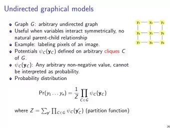
3 Probabilistic Graphical Models • Graphs endowed with a probability distribution - N odes represent random variables and the edges encode conditional independence assumptions • Graphical model express sets of conditional independence via graph structure (and conditional independence is useful) • Graph structure plus associated parameters define joint probability distribution of the set of nodes/variables Graph Probability theory theory Probabilistic graphical theory

4 Probabilistic Graphical Models • Graphical models come in two main flavors: 1. Directed graphical models (a.k.a Bayes Net, Belief Networks): - Consists of a set of nodes with arrows (directed edges) between some of the nodes - Arrows encode factorized conditional probability distributions 2. Undirected graphical models (a.k.a Markov random fields): - Consists of a set of nodes with undirected edges between some of the nodes - Edges (or more accurately the lack of edges) encode conditional independence. • Today, we will focus almost exclusively on undirected graphs.

5 PROBABILITY REVIEW: CONDITIONAL INDEPENDENCE Definition : X is conditionally independent of Y given Z if the probabil- ity distribution governing X is independent of the value of Y , given the value of Z : for all ( i, j, k ) P ( X = x i , Y = y j | Z = z k ) = P ( X = x i | Z = z k ) P ( Y = y j | Z = z k ) P ( X, Y | Z ) = P ( X | Z ) P ( Y | Z ) Or equivalently (by the product rule): P ( X | Y, Z ) = P ( X | Z ) P ( Y | X, Z ) = P ( Y | Z ) Why? Recall from the probability product rule P ( X, Y, Z ) = P ( X | Y, Z ) P ( Y | Z ) P ( Z ) = P ( X | Z ) P ( Y | Z ) P ( Z ) Example: P ( Thunder | Rain , Lightning ) = P ( Thunder | Lightning )

6 TYPES OF GRAPHICAL MODELS Probabilistic Models Graphical Models Directed Undirected

7 REPRESENTING CONDITIONAL INDEPENDENCE Some conditional independencies cannot be represented by directed graphical models: ‣ Consider 4 variables: A, B, C, D } ( A ⊥ C | B, D ) ‣ How do we represent the conditional independences: ( B ⊥ D | A, C ) A A C A B D B D D B C C ( A ⊥ C ) ( A ⊥ C | B, D ) Undirected model ( B ⊥ D | A, C ) ( B ⊥ D | A )

8 WHY UNDIRECTED GRAPHICAL MODELS? Sometime its awkward to model phenomena with directed models X 11 X 12 X 13 X 14 X 15 X 11 X 12 X 13 X 14 X 15 X 21 X 22 X 24 X 21 X 22 X 24 X 25 X 23 X 25 X 23 X 31 X 32 X 33 X 35 X 31 X 32 X 33 X 35 X 34 X 34 X 41 X 42 X 43 X 44 X 45 X 41 X 42 X 43 X 44 X 45 Image from “CRF as RNN Semantic Image Segmentation Live Demo” (http://www.robots.ox.ac.uk/~szheng/crfasrnndemo/)

9 CONDITIONAL INDEPENDENCE PROPERTIES • Undirected graphical models: ‣ Conditional independence encoded by simple graph separation. ‣ Formally, consider 3 sets of nodes: A , B and C , we say iff C x A ⊥ x B | x C separates A and B in the graph. ‣ C separates A and B in the graph: If we remove all nodes in C , there is no path from A to B in the graph. X 11 X 12 X 13 X 14 X 15 X 21 X 22 X 24 X 25 X 23 A C B

10 MARKOV BLANKET • Markov Blanket: For a given node x , the Markov Blanket is the smallest set of nodes which renders x conditionally independent of all other nodes in the graph. • Markov blanket of the 2-d lattice MRF: X 11 X 12 X 13 X 14 X 15 X 21 X 22 X 24 X 25 X 23 X 31 X 32 X 33 X 35 X 34 X 41 X 42 X 43 X 44 X 45

11 RELATING DIRECTED AND UNDIRECTED MODELS X 11 X 12 X 13 X 14 X 15 • Markov blanket of the 2-d lattice MRF: X 21 X 22 X 24 X 25 X 23 neighbours of X 23 X 31 X 32 X 33 X 35 X 34 X 41 X 42 X 43 X 44 X 45 • Markov blanket of the 2-d causal MRF: X 11 X 12 X 13 X 14 X 15 parents of X 23 X 21 X 22 X 24 X 23 X 25 children of X 23 X 31 X 32 X 33 X 35 X 34 parents of children of X 41 X 42 X 43 X 44 X 45 X 23

12 PARAMETERIZING DIRECTED GRAPHICAL MODELS Directed graphical models: • Parameterized by local conditional probability densities (CPDs) A P ( A | B ) B • Joint distributions are given as products of CPDs: N � P ( X 1 , . . . , X N ) = P ( X i | X parents(i) ) i =0

13 PARAMETERIZING MARKOV NETWORKS: FACTORS Undirected graphical models: A • Parameterized by symmetric factors or potential functions . B φ ( A, B ) - Generalizes both the CPD and the joint distribution. - Note: unlike the CPDs, the potential function are not required to normalize. • Definition : Let be a set of cliques. For each , we define a factor (also C c ∈ C called potential function or clique potential) as a nonnegative function φ c φ c ( x c ) → R where is the set of variables in clique c . x c

14 PARAMETERIZING MARKOV NETWORKS: JOINT DISTRIBUTION • Joint distribution given by a normalized product of factors: P ( x 1 , . . . , x n ) = 1 � φ c ( x c ) Z c ∈ C • Z is the partition function , it’s the normalization constant: � � Z = φ c ( x c ) c ∈ C x 1 ,...,x n • Our 4 variable example: A P ( a, b, c, d ) = 1 Z φ 1 ( a, b ) φ 2 ( b, c ) φ 3 ( c, d ) φ 4 ( d, a ) B D � Z = φ 1 ( a, b ) φ 2 ( b, c ) φ 3 ( c, d ) φ 4 ( d, a ) C a,b,c,d

15 CLIQUES AND MAXIMAL CLIQUES • What is a clique ? A subset of nodes who’s induced subgraph is complete • A maximal clique is one where you cannot add any more nodes and remain a clique A A D D B B C C Examples of maximal cliques.

16 OF GRAPHS AND DISTRIBUTIONS • Interesting fact : any positive distribution whose conditional independencies can be represented with an undirected graph can be parameterize by a product of factors ( Hammersley-Clifford theorem ). A A D D B B C C Examples of maximal cliques.

17 TYPES OF GRAPHICAL MODELS Probabilistic Models Graphical Models Directed Undirected ?

18 RELATING DIRECTED AND UNDIRECTED MODELS • What kind of probability models can be encoded by both a directed and an undirected graphical model. ➡ Answer: any probability mode whose cond. indep. relations are consistent with a chordal graph. • Chordal graph: All undirected cycles of four or more vertices have a chord. • Chord: Edge that is not part of the cycle but connects two vertices of the cycle. Not chordal: Chordal: A A A D D D B B B C C C

19 TYPES OF GRAPHICAL MODELS Probabilistic Models Graphical Models Directed Chordal Undirected

20 ENERGY -BASED MODELS • The undirected models that most interest us are energy-based models . • We reformulate the factor in log-space: φ ( x c ) φ ( x c ) = exp( − � ( x c )) or alternatively, , where . � ( x c ) = − log φ ( x c ) � ( x c ) ∈ R P ( x 1 , . . . , x n ) = 1 • Energy-based formulation of joint dist: Z exp ( − E ( x 1 , . . . , x n )) � � = 1 � E ( x 1 , . . . , x n ) is called the energy function. Z exp � c ( x c ) − c ∈ C � � where Z = exp [ − E ( x 1 , . . . , x n )] · · · x 1 x n

21 LOG-LINEAR MODEL • Log-linear models are a type of energy-based model with a particular, linear, parametrization. • In log-linear models, for clique c , the coresponding element of the energy function is composed of: � c ( x c ) 1. A parameter w c 2. A feature of the observed data f c ( x c ) � � P ( x 1 , . . . , x n ) = 1 • The joint distribution is given by � Z exp w c f c ( x c ) − c ∈ C

22 MAXIMUM LIKELIHOOD LEARNING • Maximum likelihood learning in the context of a fully observable MRF. D w ML = argmax � p ( x ( i ) ; w ) log w i =1 �� � D � log φ c ( x ( i ) = argmax c ; w c ) − log Z ( w ) w i =1 c �� D � � � � log φ c ( x ( i ) = argmax c ; w c ) − |D| log Z ( w ) w log-linear model i =1 c �� D � � � � w c f c ( x ( i ) = argmax c ) − |D| log Z ( w ) w i =1 c decomposes over the cliques does not decompose

23 MAXIMUM LIKELIHOOD LEARNING • In general, there is no closed form solution for the optimal parameters. �� � � log Z ( w ) = log exp w c f c ( x c ) x c • We can compute a gradient of the partition function. �� �� �� ∂ ∂ log Z ( w ) = log exp w c � f c � ( x c � ) ∂ w c ∂ w c c � x � x c exp ( w c f c ( x c )) f c ( x c ) = � x c exp ( � c w c f c ( x c )) = E p ( x c ; w c ) [ f c ( x c )]

24 MAXIMUM LIKELIHOOD LEARNING • The gradient of the log-likelihood �� D � � D ∂ ∂ w c � f c � ( x ( i ) � � � log p ( x ( i ) ; w ) = c � ) − D log Z ( w ) ∂ w c ∂ w c i =1 i =1 c � � D � − D ∂ � f c ( x ( i ) = c ) log Z ( w ) ∂ w c i =1 = D E p (data) [ f c ( x c )] − D E p ( x c ; w c ) [ f c ( x c )] data term model term often tractable often intractable (e.g. fully observable x ) (e.g. fully observable x )