Undirected graphical models Graph G : arbitrary undirected graph - PowerPoint PPT Presentation

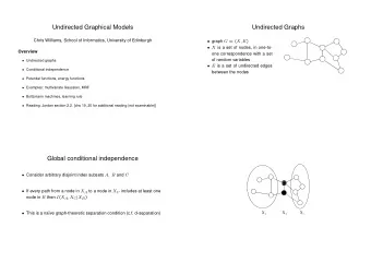
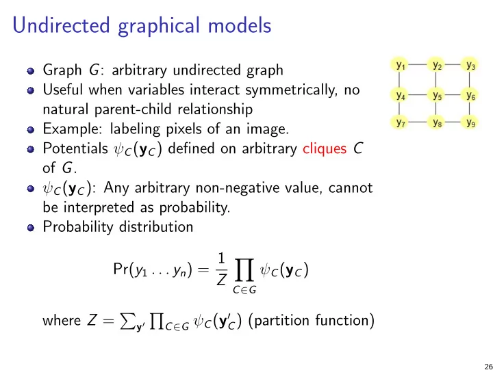
Undirected graphical models Graph G : arbitrary undirected graph Useful when variables interact symmetrically, no natural parent-child relationship Example: labeling pixels of an image. Potentials ψ C ( y C ) defined on arbitrary cliques C of G . ψ C ( y C ): Any arbitrary non-negative value, cannot be interpreted as probability. Probability distribution Pr( y 1 . . . y n ) = 1 � ψ C ( y C ) Z C ∈ G where Z = � � C ∈ G ψ C ( y ′ C ) (partition function) y ′ 26

Example y i = 1 (part of foreground), 0 otherwise. Node potentials ◮ ψ 1 (0) = 4, ψ 1 (1) = 1 ◮ ψ 2 (0) = 2, ψ 2 (1) = 3 ◮ .... ◮ ψ 9 (0) = 1, ψ 9 (1) = 1 Edge potentials: Same for all edges ◮ ψ (0 , 0) = 5, ψ (1 , 1) = 5, ψ (1 , 0) = 1 , ψ (0 , 1) = 1 Probability: Pr( y 1 . . . y 9 ) ∝ � 9 k =1 ψ k ( y k ) � ( i , j ) ∈ E ( G ) ψ ( y i , y j ) 27

Conditional independencies (CIs) in an undirected graphical model Let V = { y 1 , . . . , y n } . Local CI: y i ⊥ ⊥ V − ne ( y i ) − { y i }| ne ( y i ) 1 Pairwise CI: y i ⊥ ⊥ y j | V − { y i , y j } if edge ( y i , y j ) does not exist. 2 Global CI: X ⊥ ⊥ Y | Z if Z separates X and Y in the graph. 3 Equivalent when the distribution is positive. y 1 ⊥ ⊥ y 3 , y 5 y 6 , y 7 , y 8 , y 9 | y 2 , y 4 1 y 1 ⊥ ⊥ y 3 | y 2 , y 4 , y 5 , y 6 , y 7 , y 8 , y 9 2 y 1 , y 2 , y 3 ⊥ ⊥ y 7 , y 8 , y 9 | y 4 , y 5 , y 6 3 28

Relationship between Local-CI and Global-CI Let G be a undirected graph over V = x 1 , . . . , x n nodes and P ( x 1 , . . . , x n ) be a distribution. If P satisfies Global-CIs of G , then P will also satisfy the local-CIs of G but the reverse is not always true. We will show this with an example. Consider a distribution over 5 binary variables: P ( x 1 , . . . , x 5 ) where x 1 = x 2 , x 4 = x 5 and x 3 = x 2 A NDx 4 . Let G be x 1 x 2 x 3 x 4 x 5 All 5 local CIs in the graph: e.g. x 1 ⊥ ⊥ { x 3 , x 4 , x 5 }| x 2 etc hold in the graph. However, the global CI: x 2 ⊥ ⊥ x 4 | x 3 does not hold. 29

Relationship between Local-CI and Pairwise-CI Let G be a undirected graph over V = x 1 , . . . , x n nodes and P ( x 1 , . . . , x n ) be a distribution. If P satisfies Local-CIs of G , then P will also satisfy the pairwise-CIs of G but the reverse is not always true. We will show this with an example. Consider a distribution over 3 binary variables: P ( x 1 , x 2 , x 3 ) where x 1 = x 2 = x 3 . That is, P ( x 1 , x 2 , x 3 ) = 1 / 2 when all three are equal and 0 otherwise. Let G be x 1 x 2 x 3 All 2 pairwise CIs in the graph: e.g. x 1 ⊥ ⊥ { x 3 }| x 2 and x 2 ⊥ ⊥ { x 3 }| x 1 hold in the graph. However, the local CI: x 1 ⊥ ⊥ x 3 does not hold. 30

Factorization implies Global-CI Theorem Let G be a undirected graph over V = x 1 , . . . , x n nodes and P ( x 1 , . . . , x n ) be a distribution. If P can be factorized as per the cliques of G, then P will also satisfy the global-CIs of G Proof. Discussed in class. 31

Global-CI does not imply factorization. But global-CI does not imply factorization. Consider a distribution over 4 binary variables: P ( x 1 , x 2 , x 3 , x 4 ) Let G be x 1 x 2 x 4 x 3 Let P ( x 1 , x 2 , x 3 , x 4 ) = 1 / 8 when x 1 , x 2 , x 3 , x 4 takes values from this set = { 0000,1000,1100,1110,1111,0111,0011,0001 } . In all other cases it is zero. One can painfully check that all four globals CIs in the graph: e.g. x 1 ⊥ ⊥ { x 3 }| x 2 , x 4 etc hold in the graph. Now let us look at factorization. The factors correspond to the edges in ψ ( x 1 , x 2 ). Each of the four possible assignment of each factor will get a positive value. But that cannot represent the zero probability for cases like x 1 , x 2 , x 3 , x 4 = 0101. 32

Fractorization and CIs Theorem (Hammerseley Clifford Theorem) If a positive distribution P ( x 1 , . . . , x n ) confirms to the pairwise CIs of a UDGM G, then it can be factorized as per the cliques C of G as � P ( x 1 , . . . , x n ) ∝ ψ C ( y C ) C ∈ G Proof. Skipped. 33

Popular undirected graphical models Interacting atoms in gas and solids [ 1900] Markov Random Fields in vision for image segmentation Conditional Random Fields for information extraction Social networks Bio-informatics: annotating active sites in a protein molecules. 34

Summary Let P be a distribution and H be an undirected graph of the same set of nodes. Factorize( P , H ) = ⇒ Global-CI( P , H ) = ⇒ Local-CI( P , H ) = ⇒ Pairwise-CI( P , H ) But only for positive distributions Pairwise-CI( P , H ) = ⇒ Factorize( P , H ) Sunita Sarawagi IIT Bombay http://www.cse.iitb.ac.in/~sunita Graphical models 36 / 91

Constructing an UGM from a positive distribution using Local-CI Definition: The Markov Blanket of a variable x i , MB( x i ) is the smallest subset of variables V that makes x i CI of others given the Markov blanket. x i ⊥ ⊥ V − MB ( x i ) | MB ( x i ) The MB of a variable is always unique for a positive distribution. Sunita Sarawagi IIT Bombay http://www.cse.iitb.ac.in/~sunita Graphical models 38 / 91

Conditional Random Fields (CRFs) Used to represent conditional distribution P ( y | x ) where y = y 1 , . . . , y n forms an undirected graphical model. The potentials are defined over subset of y variables, and the whole of x . � C ψ c ( y c , x , θ ) 1 � Pr( y 1 , . . . , y n | x , θ ) = = Z θ ( x ) exp( F θ ( y c , c , x )) Z θ ( x ) c where Z θ ( x ) = � y ′ exp( � c F θ ( y ′ c , c , x )) clique potential ψ c ( y c , x ) = exp( F θ ( y c , c , x )) Sunita Sarawagi IIT Bombay http://www.cse.iitb.ac.in/~sunita Graphical models 40 / 91