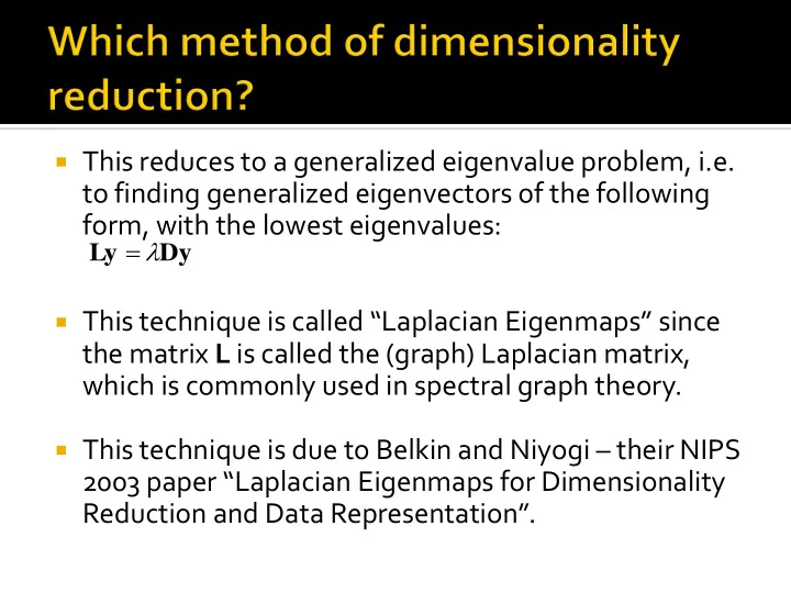
This reduces to a generalized eigenvalue problem, i.e. to finding - PowerPoint PPT Presentation
This reduces to a generalized eigenvalue problem, i.e. to finding generalized eigenvectors of the following form, with the lowest eigenvalues: Ly Dy This technique is called Laplacian Eigenmaps since the matrix L is
This reduces to a generalized eigenvalue problem, i.e. to finding generalized eigenvectors of the following form, with the lowest eigenvalues: Ly Dy This technique is called “Laplacian Eigenmaps ” since the matrix L is called the (graph) Laplacian matrix, which is commonly used in spectral graph theory. This technique is due to Belkin and Niyogi – their NIPS 2003 paper “Laplacian Eigenmaps for Dimensionality Reduction and Data Representation”.
Image source: https://people.cs.pitt.edu/~milos/co urses/cs3750/lectures/class17.pdf
Image source: https://people.cs.pitt.edu/ On this slide, N refers to the number of nearest neighbors per point ~milos/courses/cs3750/lect (the other distances are set to infinity). The parameter for the ures/class17.pdf Gaussian kernel needs to be selected carefully, especially if N is high.
We need a method of dimensionality reduction which “preserves the neighbourhood structure” of the original high dimensional points. In order words, if q i and q j were close, their lower- dimensional projections y i and y j should also be close. To define “closeness” mathematically, consider the following proximity matrix W : 2 q q Higher values for W ij means q i i j W exp and q j are nearby in the ij 2 Euclidean sense. Lower values means q i and q j are far apart.
For each of the Q tomographic projections, create a reversed copy (to take care of angles between π and 2 π ). Apply Laplacian Eigenmaps to reduce the dimensionality of these tomographic projections to 2, i.e. tomographic projection q i is mapped to y i =( 1i , 2i ), i.e. angle ϑ i = atan( 1i / 2i ). Sort the tomographic projections as per angles ϑ i Reconstruct the image based on angle estimates of the form 2 π i / Q .
Image source: Coifman et al, Graph LaplacianTomography from Unknown Random Projections
Image source: Singer and Wu, Two-dimensional tomography from noisy projections taken at unknown random directions,
For all three methods (moment-based, ordering-based, as well as based on dimensionality reduction), the tomographic projections are very noisy. They need to be denoised, for optimal performance of the algorithm.
In these applications, the projections are extremely noisy. Prior to the ordering algorithm, a denoising step is required to prevent erroneous ordering. The denoising step can be performed using Principal Components Analysis (PCA).
Assuming a Gaussian noise model, the noise variance can be semi-automatically estimated from the regions in the projections which are completely blank (modulo noise). An algorithm similar to the patch-based PCA denoising (seen in CS 663 last semester) can be employed. Given a small patch in a projection vector, we can find small patches similar to it at spatially distant locations within the same projection vector or in projection vectors acquired from other angles.
This “non - local” principle can be combined with PCA for denoising. Consider a set of clean projections { I r }, r =1 to P , corrupted by additive Gaussian noise of mean zero and standard deviation σ , to give noisy projection J r as follows: J r = I r + N r , N r ~ Gaussian distribution of mean 0 and standard deviation σ . Given each J r , we want to estimate I r , i.e. we want to denoise J r .
Consider a small p x 1 patch – denoted q ref - in some J s . Step 1: We will collect together some L patches { q 1 , q 2 ,…, q L } from { J r }, r = 1 to R , that are structurally similar to q ref – pick the L nearest neighbors of q ref . Note: even if J s is noisy, there is enough information in it to judge similarity if we assume σ << average intensity of the true projection I s . Step 2: Assemble these L patches into a matrix of size p x L . Let us denote this matrix as X ref .
T to Step 3: Find the eigenvectors of X ref X ref produce an eigenvector matrix V. Step 4: Project each of the (noisy) patches { q 1 , q 2 ,…, q L } onto V and compute their eigen- coefficient vectors denoted as { α 1 , α 2 ,…, α L } where α i = V T q i . Step 5: Now, we need to manipulate the eigencoefficients of q ref in order to denoise it.
Step 5 (continued): We will follow a Wiener filter type of update: 1 β α 2 ( l ) ( l ), 0 l p 1 Noise variance (assumed known or can be ref ref 2 1 estimated) α 2 ( l ) Estimate of coefficient squared of true signal α Note : is a vector of eigencoeff icients of the reference (noisy) patch and contains ref α β p elements, of which the l - th element is ( l ). is the vector of eigencoeff icients ref ref of the filtered patch. L 1 α 2 2 2 ( l ) max( 0 , i l ( ) ) L i 1 Why this formula? We will see later. Step 6: Reconstruct the reference patch as follows: q V β denoised ref ref
Repeat steps 1 to 6 for all p x 1 patches from image J (in a sliding window fashion). Since we take overlapping patches, any given pixel will be covered by multiple patches (as many as p different patches). Reconstruct the final projection by averaging the output values that appear at any pixel.
Note that a separate eigenspace is created for each reference patch. The eigenspace is always created from patches that are similar to the reference patch. Such a technique is often called as spatially varying PCA or non-local PCA .
To compute L nearest neighbors of q ref , restrict your search to a window around q ref . For every patch within the window, compute the sum of squared differences with q ref , i.e. p 2 compute: . ( q ( i ) s ( i )) ref i 1 Pick L patches with the least distance.
Eigen- coefficients of the “true patch”. We are 2 ( l ) k ( l ) ( l ), 0 l p 1 i i looking for a linear update which motivates 2 this equation. k * arg min E ( ( l ) k ( l ) ( l )) k ( l ) i i 2 2 2 arg min E (( ( l )) k ( l ) ( l ) 2 k ( l ) ( l ) ( l )) k ( l ) i i i i n i represents a vector of pure noise q q n q q n values which degrades the true noisy true T noisy T true : ( ) Consider V V patch to give the noisy patch. Its i i i i i i projection onto the eigenspace gives ( l ) ( l ) ( l ) i i i vector ϒ i . We will drop the index l and subscript i for better readabilit y : 2 2 2 k * arg min E ( k 2 k ) k 2 2 2 arg min E ( k ( ) 2 k ( )) k 2 2 2 2 2 arg min E ( ) k E ( ) 2 kE ( ), as E ( ) E ( ) E ( ) 0 k T T since E ( ) E ( V n ) V E ( n ) 0 As the image and the noise are independent As the noise is zero mean
Setting derivative w.r.t. k to 0, we get 2 2 E ( ) E ( ) 2 2 2 kE ( ) E ( ) k 2 2 2 2 E ( ) E ( ) 2 How should we estimate ( ) ? E Re call : Since we are dealing with ( l ) ( l ) ( l ) ( l ) ( l ) L similar patches, we can i i i i assume (approximately) 2 2 2 that the l -th eigen- E ( ( l )) E ( ( l )) E ( ( l )) i i coefficient of each of 2 2 2 E ( ( l )) E ( ( l )) i those L patches are very L 1 similar. 2 2 ( l ) i L i 1 This may be a negative value, so we set it to be L 1 2 2 2 E ( ( l )) max( 0 , ( l ) ) i L i 1
Image source: Singer and Wu, Two- dimensional tomography from noisy projections taken at unknown random directions
Image source: Singer and Wu, Two-dimensional tomography from noisy projections taken at unknown random directions
Image source: Singer and Wu, Two- dimensional tomography from noisy projections taken at unknown random directions
The planes of projection in directions d i and d j will intersect in a common line c ij . Hence their corresponding central slices through the Fourier volume will also have a common line . The common line can be determined by a search in the Fourier space! Ajit Rajwade
Central Fourier planes corresponding to directions d i and d j v r i =F(R di f ) u v r j =F(R dj f ) u Intersection of the planes in the Fourier space leads to a common line. The directions of projection are unknown, but the common line can be found out by searching over pairs of directions in the Fourier space and finding the best match. Ajit Rajwade
Recommend
More recommend
Explore More Topics
Stay informed with curated content and fresh updates.
