ECS 231 Gradient descent methods for solving large scale eigenvalue - PowerPoint PPT Presentation
ECS 231 Gradient descent methods for solving large scale eigenvalue problems 1 / 17 Generalized symmetric definite eigenvalue problem Generalized symmetric definite eigenvalue problem Au = Bu where A and B are n n symmetric, and B
ECS 231 Gradient descent methods for solving large scale eigenvalue problems 1 / 17
Generalized symmetric definite eigenvalue problem ◮ Generalized symmetric definite eigenvalue problem Au = λBu where A and B are n × n symmetric, and B positive definite, ◮ All eigenvalues and eigenvectors are real ◮ Denote the eigenvalues by λ 1 ≤ λ 2 ≤ · · · ≤ λ n and their associated eigenvectors by u 1 , u 2 , . . . , u n and u i are normalized, i.e., � u i � B = 1 for i = 1 , 2 , . . . , n ◮ � · � B is defined through the B -inner product � x, y � B = � Bx, y � ≡ y T Bx. 2 / 17
Rayleigh quotient and minimization principles ◮ Rayleigh Quotient is defined by ρ ( x ) = x T Ax x T Bx ◮ Minimization principle: λ 1 = λ min = min x ρ ( x ) u 1 = argmin x ρ ( x ) ◮ In general for i > 1 λ i = x ⊥ B u j , 1 ≤ j<i ρ ( x ) min u i = argmin x ⊥ B u j , 1 ≤ j<i ρ ( x ) where by x ⊥ B y we mean that � x, y � B = 0 . 3 / 17
Optimization methods for eigen-computation ◮ By the minimization principles, various optimization techniques can be naturally employed to compute λ 1 or the first few λ i and their associated eigenvectors. ◮ Gradient (steepest) Decent (GD) and Conjugate Gradient (CG) methods are based on minimizing the Rayleigh Quotient ρ ( x ) . ◮ Two useful quantities: ◮ The gradient of ρ ( x ) : 2 2 ∇ ρ ( x ) = x T Bx [ Ax − ρ ( x ) Bx ] = x T Bxr ( x ) ◮ The Hessian of ρ ( x ) : 2 x T Bx [ A − ρ ( x ) B − ∇ ρ ( x )( Bx ) T − ( Bx ) ∇ ρ ( x ) T ] ∇ 2 ρ ( x ) = 4 / 17
Line search ◮ Minimizing the Rayleigh quotient along the direction of the gradient r = r ( x ) is equivalently to solve the single-variable optimization problem min ρ ( x + tr ) = ρ ( x + t opt r ) t 5 / 17
Steepest decent (SD) method One step of the SD: ◮ Given an approximation x to u 1 and � x � B = 1 ◮ Compute the search direction: the (opposite) direction of the gradient r = ∇ ρ ( x ) , ◮ solve the problem inf t ρ ( x + tr ) = ρ ( x + t opt r ) ◮ update x := x + t opt r. 6 / 17
Steepest decent (SD) method Given an initial approximation x 0 to u 1 , and a relative tolerance rtol , the algorithm attempts to compute an approximate pair to ( λ 1 , u 1 ) with the prescribed rtol . 1 x 0 = x 0 / � x 0 � B , ρ 0 = x T 0 Ax 0 , r 0 = Ax 0 − ρ 0 Bx 0 2 for i = 0 , 1 , . . . , do 3 if � r i � / ( � Ax i � 2 + | ρ i | � Bx i � 2 ) ≤ rtol , break 4 solve inf t ρ ( x i + tr i ) for t opt 5 � x = x i + t opt r i , x i +1 = � x/ � � x � B ρ i +1 = x T 6 i +1 Ax i +1 , r i +1 = Ax i +1 − ρ i +1 Bx i +1 7 end 8 return ( ρ i , x i ) as an approximate eigenpair to ( λ 1 , u 1 ) 7 / 17
Steepest decent (SD) method Alternatively , the SD method can also be reformulated under Rayleigh-Ritz subspace projection framework: 1 select initial vector x 0 , and compute ρ 0 = ρ ( x 0 ) 2 for i = 0 , 1 , . . . until convergence do 3 compute r i = Ax i − ρ i Bx i compute H = Z T AZ and S = Z T BZ , where Z = [ x i , r i ] 4 5 compute the smallest eigenpair ( γ 1 , w 1 ) of ( H, S ) 6 update ρ i +1 = γ 1 , x i +1 = Zw 1 7 end 8 return ( ρ i , x i ) as an approximate eigenpair to ( λ 1 , u 1 ) 8 / 17
Steepest decent (SD) method Remarks: 1. Convergence analysis ◮ The case B = I , locally , the convergence rate is � 2 � 1 − ξ ρ i +1 − λ 1 ξ = λ 2 − λ 1 ∼ , λ n − λ 1 . ρ i − λ 1 1 + ξ [Faddeev and Faddeeva’63] and [Knyazev and Skorokhodov’91] : ◮ For the case B � = I , [Yang’93]. 2. Entending the search space ρ new = z ∈ span { x i ,r i } ρ ( z ) min ⇓ ρ new = z ∈ K m ( A − ρ i B,x i ) ρ ( z ) min 9 / 17
Steepest decent (SD) method 3. Preconditioning the search direction r i ⇒ K i r i where K i is a preconditioner (more later) 4. Introducing block implementation R ( X ) = [ r ( x ( i ) 1 ) , r ( x ( i ) 2 ) , . . . , r ( x ( i ) k )] Further reading: R.-C. Li, Rayleigh quotient based optimization methods for eigenvalue problems, in “Matrix Functions and Matrix Equations”, Z. Bai et al ed., World Scientific, 2015. 10 / 17
Conjugate gradient method ◮ The Conjugate Gradient (CG) method was originally proposed in 1950s by Hestenes and Stiefel for solving linear system Hx = b where H is symmetric positive definite. ◮ In the 1960s, it was extended by Fletcher and Reeves as an iterative method for nonlinear optimization problems. The extension is almost verbatim. ◮ Because of the optimality properties of Rayleigh quotients, it is natural to apply the CG method to compute a few eigenpairs of A − λB . 11 / 17
CG for linear systems: review ◮ Define φ ( x ) = 1 2 x T Hx − x T b. (1) ◮ the gradient ∇ φ ( x ) = Hx − b = r ( x ) (the residual vector) the Hessian matrix H ( x ) = H . ◮ φ ( x ) is a quadratic functional in x . It is convex and has a unique local and global minimum at x = H − 1 b . ◮ Given an initial guess x 0 , the CG method iteratively produces a sequence of approximations x i and p i , such that φ ( x i +1 ) = min α φ ( x i + αp i ) . where p i are conjugate searching directions, i.e., p T i Hp j = 0 for i � = j , and p 0 = r ( x 0 ) . 12 / 17
CG for linear systems: review CG algorithm: 1. Give an initial guess x 0 , compute r 0 = Ax 0 − b , and set p 0 = r 0 ; 2. For i = 0 , 1 , . . . , do α i = argmin α φ ( x i + αp i ) = r T i Ar i p T i Ap i x i +1 = x i + α i p i r i +1 = r i − α i Hp i β i = r T i +1 r i +1 r T i r i p i +1 = r i +1 + β i p i Note that β i is chosen so that p T i +1 Hp i = 0 . 13 / 17
CG for linear systems: review ◮ In the absence of roundoff errors, it can be proved that 1. r T i r j = 0 , for 0 ≤ i, j ≤ ℓ and i � = j 2. subspan { r 0 , r 1 , . . . , r ℓ } = subspan { p 0 , p 1 , . . . , p ℓ } = subspan { r 0 , Hr 0 , . . . , H ℓ r 0 } 3. p 0 , p 1 , . . . , p ℓ are linearly independent and p T i Hp j = 0 , for 0 ≤ i, j ≤ ℓ and i � = j 4. φ ( x ℓ ) = min t 0 ,...,t ℓ φ ( x 0 + t 0 p 0 + t 1 p 1 + · · · + t ℓ p ℓ ) . ◮ The CG method converges in at most n steps, a direct method , is a consequence of these properties. 14 / 17
CG method for eigenvalue computation ◮ In extending the CG method, the key is to recognize that the residual r ( x ) in the linear system case plays the role of the gradient direction for φ ( x ) . ◮ For the eigenproblem of A − λB , the objective function is the Rayleigh quotient ρ ( x ) = x T Ax x T Bx whose gradient ∇ ρ ( x ) is collinear to r ( x ) = Ax − ρ ( x ) Bx. 15 / 17
CG method for eigenvalue computation Given an initial approximation x 0 to u 1 , and a relative tolerance rtol , the algorithm attempts to compute an approximate pair to ( λ 1 , u 1 ) with the prescribed rtol . x 0 = x 0 / � x 0 � B , ρ 0 = x T 1 0 Ax 0 , r 0 = Ax 0 − ρ 0 Bx 0 , p 0 = r 0 ; 2 for i = 0 , 1 , . . . , do 3 if � r i � / ( � Ax i � 2 + | ρ i | � Bx i � 2 ) ≤ rtol , break; 4 solve inf t ρ ( x i + tp i ) = ρ ( x i + t opt p i ) . 5 α i = t opt 6 ˆ x = x i + α i p i , x i +1 = ˆ x/ � ˆ x � B ; ρ i +1 = x T 7 i +1 Ax i +1 , r i +1 = Ax i +1 − ρ i +1 Bx i +1 , 8 choose β i and update p i +1 = r i +1 + β i p i , 9 endfor 10 Return ( ρ i , x i ) as an approximate eigenpair to ( λ 1 , u 1 ) . 16 / 17
Conjugate gradient method ◮ Different choice of β i leads to the different version of the CG method. Common choices: β i = r T β i = r T i +1 r i +1 i +1 ( r i +1 − r i ) or r T r T i r i i r i ◮ Choose β i , together with α i , to minimize the Rayleigh quotient on the projection subspace subspan { x i +1 , r i +1 , p i } = subspan { x i +1 , r i +1 , x i } leads to the locally optimal method. – the state of the art? Ref.: A. Knyazev, Toward the optimal preconditioned eigensolver: locally optimal block preconditioned conjugate gradient method. SIAM J. Sci. Comput. 23(2):517-541, 2001 ◮ Open problem: no quantitative estimate on the convergence rate of the CG method is available yet. 17 / 17
Recommend
More recommend
Explore More Topics
Stay informed with curated content and fresh updates.
