This reduces to a generalized eigenvalue problem, i.e. to finding - - PowerPoint PPT Presentation

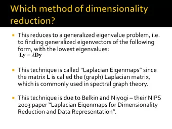
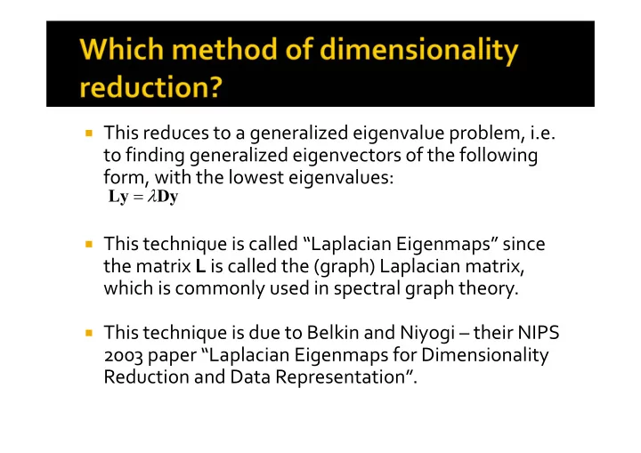
 This reduces to a generalized eigenvalue problem, i.e.

to finding generalized eigenvectors of the following form, with the lowest eigenvalues:

 This technique is called “Laplacian Eigenmaps” since

the matrix L is called the (graph) Laplacian matrix, which is commonly used in spectral graph theory.

 This technique is due to Belkin and Niyogi – their NIPS

2003 paper “Laplacian Eigenmaps for Dimensionality Reduction and Data Representation”.

Dy Ly  

On this slide, N refers to the number of nearest neighbors per point (the other distances are set to infinity). The parameter  for the Gaussian kernel needs to be selected carefully, especially if N is high.

Image source: https://people.cs.pitt.edu/ ~milos/courses/cs3750/lect ures/class17.pdf

        

 In these applications, the projections are

extremely noisy.

 Prior to the ordering algorithm, a denoising

step is required to prevent erroneous

• rdering.

 The denoising step can be performed using

Principal Components Analysis (PCA).

 Repeat steps 1 to 6 for all p x 1 patches from

image J (in a sliding window fashion).

 Since we take overlapping patches, any given

pixel will be covered by multiple patches (as many as p different patches).

 Reconstruct the final projection by averaging

the output values that appear at any pixel.

 Assuming a Gaussian noise model, the noise

variance can be semi‐automatically estimated from the regions in the projections which are completely blank (modulo noise).

 An algorithm similar to the patch‐based PCA

denoising (seen in CS 663 last semester) can be employed.

 Given a small patch in a projection vector, we

can find small patches similar to it at spatially distant locations within the same projection vector or in projection vectors acquired from

• ther angles.

2 2 2 2 2 2 2 2 2

) ( ) ( ) ( ) ( ) ( ) ( get we 0, to w.r.t. derivative Setting                 E E E E k E kE k ) ( ) ( ) ( ) ( ) ( : Re ? ) ( estimate we should How

2

l l l l l call E

i i i i

          Since we are dealing with L similar patches, we can assume (approximately) that the l‐th eigen‐ coefficient of each of those L patches are very similar. ) ) ( 1 , max( )) ( ( be it to set we so value, negative a be may This ) ( 1 )) ( ( )) ( ( )) ( ( )) ( ( )) ( (

2 1 2 2 2 1 2 2 2 2 2 2 2

                    

 

  L i i L i i i i i

l L l E l L l E l E l E l E l E

 In this case, the image f is in 3D and each

tomographic projection is in 2D.

 Per Fourier slice theorem, 2D Fourier

transform of a 2D projection in direction d is equal to the central slice through the 3D Fourier transform of f.

 But in 3D we actually have some more

information – which is absent in 2D!

Ajit Rajwade

 The planes of projection in directions di and dj

will intersect in a common line cij.

 Hence their corresponding central slices

through the Fourier volume will also have a common line.

 The common line can be determined by a

search in the Fourier space!

Ajit Rajwade

Ajit Rajwade

v u v u Intersection of the planes in the Fourier space leads to a common line. The directions of projection are unknown, but the common line can be found out by searching over pairs of directions in the Fourier space and finding the best match. ri=F(Rdif) rj=F(Rdjf) Central Fourier planes corresponding to directions di and dj

 Consider the following equation:

Ajit Rajwade

) , sin , (cos

ij ij

   

ij ij i

b c R

Common line in global coordinate system Common line expressed in local coordinate system of plane of projection in direction di

2 ,

) ( ) ( min arg ) , (    

  j i

r r  

ji ij

Angle made by cij with local X axis

 We see that  Consider viewing directions c12, c23, c31. Then

we have

Ajit Rajwade

ik ij ik i ij i ik ij ij ij i

c c c R c R b b b c R          ) cos( ) , sin , (cos

ik ij ij ij

   

             

                   1 cos cos cos 1 cos cos cos 1 ,

13 12 21 23 13 12 32 31 21 23 32 31

            M CC M c c c C

31 23 12 T

 The matrix C is rank 3 in the case that the

common lines are not coplanar.

 To obtain C from M, we have

Ajit Rajwade

ambiguity) eflection rotation/r (upto

5 .

UD C UDU CC M    

T T

M will be positive semi‐definite with unit diagonal entries

 We have the following relation:

Ajit Rajwade

i i i

B C R 

This is a 3 X (Q‐1) matrix

• f common lines

involving the i‐th

• projection. The lines are

expressed in global coordinate system This is a 3 X (Q‐1) matrix

• f common lines

involving the i‐th

• projection. The lines are

expressed in the local coordinate system of the i‐th plane

 To estimate Ri:

Ajit Rajwade

T T T T F

I E UV R USV C B R R B C R R

i i

i i i i i i i

    

• f

SVD he Consider t : Solution that such ) (

T 2

See class handout for more details of this solution!

 For all pairs of directions (di,dj) find the angle φij.  For the i‐th direction, assemble the matrix Bi and

the matrix Mi using the knowledge of the angles φij.

 Use eigenvalue decomposition on Mi to get Ci.  Use the SVD method to obtain Ri from Ci and Bi.  Repeat this for all i.  That gives us the directions of tomographic

projection!

Ajit Rajwade

 Consider a piecewise constant signal f

(having length n). Suppose coefficients of f are measured through the measurement matrix  yielding a vector y of only m << n measurements. If (C is some constant) then the solution to the following is exact with probability :

f y f TV

T f

  such that ) ( min

n m R f R R y

n n m m

    



, , , ) , ( ) / log(

2

      n C m

Ref: Candes, Romberg and Tao, “Robust Uncertainty Principles: Exact Signal Reconstruction from Highly Incomplete Frequency Information”, IEEE Transactions on Information Theory, Feb 2006.

 Define vector h as follows:  So we will do the following:

C C

C C C

set from ts coefficien frequency

• nly those

selects which by | | size

• f

matrix ) 1 ( ) ( for which matrix diagonal

• f

ts coefficien Fourier where that such min arg *

1 2 1

N

• e

u,u D

• πu/N
• j

T T

        I D h h Ψ Ah h DΨ I DH I G h h

h

) ( ) 1 ( ) ( ) 1 ( ) ( ) (

/ 2

u F e u H x f x f x h

N u j  

     

             w.r.t. minimize

2 F T T

ΦV

T m)

| ... | | ( ) ,..., , diag( Consider

2 1 n 2 1

          ) ,..., , ( where

, 2 , 2 1 , 1 2 2 n i n i i i F j i t j j t i i F T

                   





Rank one matrix Ej We want a rank one matrix that approximates Ej as closely as possible in the Frobenius sense. The solution lies in SVD!

 This method does not directly target  but

instead considers the Gram matrix DTD where

 The aim is to design Φ in such a way that the

Gram matrix resembles the identity matrix as much as possible, in other words we want:

. normalized

• unit

columns all with ΦΨ D  I ΦΨ Φ Ψ 

T T

) ,..., , ( where

, 2 , 2 1 , 1 2 2 n i n i i i F j i t j j t i i F T

                   





Rank one matrix Ej We want a rank one matrix that approximates Ej as closely as possible in the Frobenius sense. The solution lies in SVD.

t j t k k k kk T j

u S u u S USU E

1 11

  





Assuming that S11 is the largest singular value