The modelling of tidal turbine farms using multi-scale, unstructured - - PowerPoint PPT Presentation

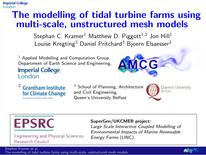
The modelling of tidal turbine farms using multi-scale, unstructured mesh models

Stephan C. Kramer1 Matthew D. Piggott1,2 Jon Hill1 Louise Kregting3 Daniel Pritchard3 Bjoern Elsaesser3

1 Applied Modelling and Computation Group,

Department of Earth Science and Engineering, 2

3 School of Planning, Architecture

and Civil Engineering, Queen’s University Belfast SuperGen/UKCMER project: Large Scale Interactive Coupled Modelling of Environmental Impacts of Marine Renewable Energy Farms (LINC)

Stephan Kramer et al. The modelling of tidal turbine farms using multi-scale, unstructured mesh models

Outline

◮ Benchmarking of Fluidity and MIKE 21 in a simplified

tidal basin geometry.

◮ Implementation of turbines in coarse resolution tidal

models.

◮ Correction to drag coefficient to avoid incorrect mesh

dependence

Stephan Kramer et al. The modelling of tidal turbine farms using multi-scale, unstructured mesh models

http://amcg.ese.ic.ac.uk/fluidity Open Source Finite Element Modelling framework used for a variety of Earth sci- ence and engineering applcations. Fluidity solves 3D non-hydrostatic Navier Stokes equations, but also depth-averaged 2D shallow water equations. It implements a host of advanced numerical techniques, e.g. mesh adaptivity which dynamically adapts the mesh to focus resolution where needed. In development: optimisation framework for farm layouts

Stephan Kramer et al. The modelling of tidal turbine farms using multi-scale, unstructured mesh models

http://amcg.ese.ic.ac.uk/fluidity Open Source Finite Element Modelling framework used for a variety of Earth sci- ence and engineering applcations. Fluidity solves 3D non-hydrostatic Navier Stokes equations, but also depth-averaged 2D shallow water equations. It implements a host of advanced numerical techniques, e.g. mesh adaptivity which dynamically adapts the mesh to focus resolution where needed. In development: optimisation framework for farm layouts Widely used in marine engineering.

◮ 3D and 2D capability (MIKE 3, MIKE 21) ◮ Sediment transport ◮ Ecological modelling (ECO Lab) ◮ Wetting and drying ◮ Structures (including turbines!)

Stephan Kramer et al. The modelling of tidal turbine farms using multi-scale, unstructured mesh models

Tidal basin benchmark

Idealised tidal basin based on Strangford Lough. Tidal forcing through periodic free surface elevation on the left open

• boundary. For now: fixed eddy viscosity (10 m2/s). Idealised
• bathymetry. Both models use the same triangular meshes.

Stephan Kramer et al. The modelling of tidal turbine farms using multi-scale, unstructured mesh models

Comparison in tidal basin - Flood

Fluidity - Shallow Water Equations MIKE 21

Stephan Kramer et al. The modelling of tidal turbine farms using multi-scale, unstructured mesh models

Convergence of numerical results

Integrated L2-norm difference between model results at various mesh resolutions and at finest resolution (∆x = 31.25 m). Blue shows the convergence of Fluidity’s results to its finest resolution result, and green the convergence of MIKE’s results to its finest resolution. Red shows the convergence of MIKE’s results to the finest resolution Fluidity results.

Stephan Kramer et al. The modelling of tidal turbine farms using multi-scale, unstructured mesh models

Velocity over time at a fixed

• point. Plotted here is u3; This

will determine energy yield of a turbine at this point.

Stephan Kramer et al. The modelling of tidal turbine farms using multi-scale, unstructured mesh models

Temporal average

Convergence of temporal average of u3 at a fixed point.

Stephan Kramer et al. The modelling of tidal turbine farms using multi-scale, unstructured mesh models

Parameterisation of turbines in SWE models

Total body drag force on turbine:

• F(

u) = 1

2ρ0CD(u)Acrossu

u Represented as a momentum source f( u): Depth avg. momentum eqn.: ρ0 ∂ u ∂t +ρ0 u· ∇ u+g ∇η+· · · = f( u) Applied over some horizontal area A, we need:

• A
• f(

u) =

• A
• F(u)

AH =

• A

ρ0CD(u)Across 2AH u u Therefore, we end up with a quadratic “bottom” drag force:

• f(

u) = ρ0CD(u)Across 2AH u u

Stephan Kramer et al. The modelling of tidal turbine farms using multi-scale, unstructured mesh models

Turbines in Fluidity and MIKE

Fluidity MIKE 21 Visualisation of wake by velocity deficit (difference between solution with and without a turbine). Note that we do not expect a realistic wake as no turbulence model is used (fixed eddy viscosity).

Stephan Kramer et al. The modelling of tidal turbine farms using multi-scale, unstructured mesh models

Turbines in Fluidity and MIKE

Turbines at coarse resolution are represented as point momentum sources. This means the finer the resolution, the smaller the area the drag is applied over. Leads to mesh dependency when resolving close to the turbine scale.

Stephan Kramer et al. The modelling of tidal turbine farms using multi-scale, unstructured mesh models

Drop in local velocity

∆x = 320 ∆x = 160 ∆x = 80 ∆x = 40 ∆x = 20 ∆x = 10 ∆x = 5 ∆x = 2 ∆x = 1 Resolution ∆x in m 2.00 2.20 2.40 2.60 2.80 3.00 3.05 Speed (m/s)

upstream speed local speed MIKE local speed Fluidity

Local velocity in cell containing the turbine, drops significantly with increasing resolution. This local velocity is used to compute the drag force to be applied and the energy yield.

Stephan Kramer et al. The modelling of tidal turbine farms using multi-scale, unstructured mesh models

Drop in local velocity

∆x = 320 ∆x = 160 ∆x = 80 ∆x = 40 ∆x = 20 ∆x = 10 ∆x = 5 ∆x = 2 ∆x = 1 Resolution ∆x in m 2.00 2.20 2.40 2.60 2.80 3.00 3.05 Speed (m/s)

upstream speed local speed MIKE local speed Fluidity local speed LMADT

For resolution near the turbine scale (turbine diameter here is D = 16 m), the local velocity in cell matches the local turbine velocity predicted by actuator disc theory (LMADT).

Stephan Kramer et al. The modelling of tidal turbine farms using multi-scale, unstructured mesh models

Drop in local velocity

∆x = 320 ∆x = 160 ∆x = 80 ∆x = 40 ∆x = 20 ∆x = 10 ∆x = 5 ∆x = 2 ∆x = 1 Resolution ∆x in m 2.00 2.20 2.40 2.60 2.80 3.00 3.05 Speed (m/s)

upstream speed local speed MIKE local speed Fluidity local speed LMADT predicted speed

For resolutions larger than the turbine scale, the local velocity can be predicted by a modified actuator disc theory taking into account the length scale, ∆x, over which the force is applied.

Stephan Kramer et al. The modelling of tidal turbine farms using multi-scale, unstructured mesh models

u0 u0 u0 u4 u3 u4 u1 ∆y Adjust actuator disc theory (see Garret and Cummins ’07), to take into account that the drag force F = 1

2ρ0CD(u)Acrossu2,

is not applied over the width of the turbine (diameter D), but

• ver the width, ∆y, of the cell the drag is applied within.

Stephan Kramer et al. The modelling of tidal turbine farms using multi-scale, unstructured mesh models

Correction in drag coefficient

Using the modified theory we can express the drag as a function of the local cell velocity instead of the upstream velocity: F = 1

2ρwCT

4

• 1 + √1 − γ

2Acrossulocal2, where γ = CT Across ∆yH . Here ∆yH is the modified cross section, the product of the cell width ∆y and water depth H. In 3D, if we ignore the difference between the cell width and the turbine diameter, we have γ = CT and we recover the correction by Roc et al. ’13. This assumes we resolve the turbine scale.

Stephan Kramer et al. The modelling of tidal turbine farms using multi-scale, unstructured mesh models

Correction in drag coefficient

∆x = 320 ∆x = 160 ∆x = 80 ∆x = 40 ∆x = 20 ∆x = 10 Resolution ∆x in m 460 480 500 520 540 560 580 Force (kN)

analytical force force MIKE force Fluidity force Fluidity with correction

Without correction, the drag force applied in the model drops significantly with resolution (up to 75 kN). With correction the change in applied force is limited (less than 12kN).

Stephan Kramer et al. The modelling of tidal turbine farms using multi-scale, unstructured mesh models

Conclusions:

◮ Study of hydrodynamic capabilities of MIKE 21 and Fluidity,

for the tidal modelling of turbine farms with an application of energy resource and environmental impact assessments.

◮ Turbine drag parameterisation implemented as a point

momentum source is mesh dependent and leads to an incorrect drag force for resolutions close to the turbine scale.

◮ Using actuator disc theory the drag coefficient can be

corrected such that the correct force is applied.

Future work:

◮ Study capabilities for environmental impact

studies: modelling biology with tracer fields, particles, and species interactions (ECO Lab).

◮ Improved wake representation through

turbulence modelling. Comparison with 3D CFD and lab results.

Stephan Kramer et al. The modelling of tidal turbine farms using multi-scale, unstructured mesh models