Students t -distribution STAT 587 (Engineering) Iowa State - PowerPoint PPT Presentation
Students t -distribution STAT 587 (Engineering) Iowa State University September 17, 2020 Students t distribution Probability density function Students t distribution The random variable X has a Students t distribution with degrees of
Student’s t -distribution STAT 587 (Engineering) Iowa State University September 17, 2020
Student’s t distribution Probability density function Student’s t distribution The random variable X has a Student’s t distribution with degrees of freedom ν > 0 if its probability density function is � ν +1 � − ν +1 � p ( x | ν ) = Γ � 1 + x 2 2 2 √ νπ Γ( ν 2 ) ν where Γ( α ) is the gamma function, � ∞ x α − 1 e − x dx. Γ( α ) = 0 We write X ∼ t ν .
Student’s t distribution Probability density function - graphically Student’s t probability density function Student's t random variables 0.4 Probablity density function, p(x) 0.3 Degrees of freedom 1 0.2 10 100 0.1 0.0 −4 −2 0 2 4 x
Student’s t distribution Mean and variance Student’s t mean and variance If T ∼ t v , then � ν +1 � ∞ � − ν +1 � x Γ � 1 + x 2 2 2 E [ X ] = √ νπ Γ( ν dx = · · · = 0 , ν > 1 ν 2 ) −∞ and � ν +1 � ∞ � − ν +1 � ( x − 0) 2 Γ 1 + x 2 � ν 2 2 V ar [ X ] = √ νπ Γ( ν dx = · · · = ν − 2 , ν > 2 . 2 ) ν 0
Student’s t distribution Cumulative distribution function - graphically Gamma cumulative distribution function - graphically Student's t random variables 1.00 Cumulative distribution function, F(x) 0.75 Degrees of freedom 1 0.50 10 100 0.25 0.00 −4 −2 0 2 4 x
Generalized Student’s t distribution Location-scale t distribution Location-scale t distribution If X ∼ t ν , then Y = µ + σX ∼ t ν ( µ, σ 2 ) for parameters: degrees of freedom ν > 0 , location µ and scale σ > 0 . By properties of expectations and variances, we can find that E [ Y ] = µ, ν > 1 and ν ν − 2 σ 2 , V ar [ Y ] = ν > 2 .
Generalized Student’s t distribution Probability density function Generalized Student’s t probability density function The random variable Y has a generalized Student’s t distribution with degrees of freedom ν > 0 , location µ , and scale σ > 0 if its probability density function is � 2 � − ν +1 � ν +1 � � Γ 2 1 + 1 � y − µ 2 p ( y ) = 2 ) √ νπσ Γ( ν ν σ We write Y ∼ t ν ( µ, σ 2 ) .
Generalized Student’s t distribution Probability density function - graphically Generalized Student’s t probability density function Student's t 10 random variables 0.4 Probablity density function, p(x) 0.3 Scale, σ 1 2 0.2 Location, µ 0 2 0.1 0.0 −4 −2 0 2 4 x
Generalized Student’s t distribution t with 1 degree of freedom t with 1 degree of freedom If T ∼ t 1 ( µ, σ 2 ) , then T has a Cauchy distribution and we write T ∼ Ca ( µ, σ 2 ) . If T ∼ t 1 (0 , 1) , then T has a standard Cauchy distribution. A Cauchy random variable has no mean or variance.
Generalized Student’s t distribution As degrees of freedom increases As degrees of freedom increases If T ν ∼ t ν ( µ, σ 2 ) , then d = X ∼ N ( µ, σ 2 ) ν →∞ T ν lim
Generalized Student’s t distribution t distribution arise from a normal sample t distribution arising from a normal sample iid ∼ N ( µ, σ 2 ) . We calculate the sample mean Let X i n X = 1 � X i n i =1 and the sample variance n 1 S 2 = � ( X i − X ) 2 . n − 1 i =1 Then T = X − µ S/ √ n ∼ t n − 1 .
Generalized Student’s t distribution Inverse-gamma scale mixture of a normal Inverse-gamma scale mixture of a normal If � ν 2 , ν X | σ 2 ∼ N ( µ, σ 2 /n ) σ 2 ∼ IG 2 s 2 � and then X ∼ t ν ( µ, s 2 /n ) which is obtained by � p x | σ 2 ( x | σ 2 ) p σ 2 ( σ 2 ) dσ 2 p x ( x ) = where p x is the marginal density for x p x | σ 2 is the conditional density for x given σ 2 , and p σ 2 is the marginal density for σ 2 .
Generalized Student’s t distribution Summary Summary Student’s t random variable: T ∼ t ν ( µ, σ 2 ) , ν, σ > 0 E [ X ] = µ, ν > 1 ν − 2 σ 2 , ν > 2 ν V ar [ X ] = Relationships to other distributions
Recommend
More recommend
Explore More Topics
Stay informed with curated content and fresh updates.

