Exponential & Normal Distribution Lec.22 July 29, 2020 - PowerPoint PPT Presentation

Exponential & Normal Distribution Lec.22 July 29, 2020

Exponential Distribution: Fundamental Idea The exponential distribution is the continuous analog of the geometric distribution. In the case of the geometric coin flipping experiment, we know that the first Heads occurs at a discrete point in time. In the real-world, we might be waiting for a system to crash, or for a Piazza question to be answered. Here we have a continuous point in time, as opposed to a discrete one. These scenarios are naturally modeled by the exponential distribution.

Definition For λ > 0, a a continuous random variable X with pdf ( λ e − λ x , if x ≥ 0 f ( x ) = 0 , otherwise is called an exponential random variable with rate parameter λ , and we write X ∼ Exp ( λ )

Picture

Check

Check f ( x ) is nonnegative. Furthermore Z ∞ Z ∞ λ e − λ x dx = − e − λ x | ∞ f ( x ) dx = 0 = 0 − ( − 1) = 1 0 −∞ Thus, f ( x ) is a valid pdf.

Mean and Variance of an Exponential

Mean and Variance of an Exponential X ∼ Exp ( λ ) Z ∞ x λ e − λ x dx = 1 E [ X ] = λ 0 Z ∞ x 2 λ e − λ x dx = 2 E [ X 2 ] = λ 2 0 Var ( X ) = E [ X 2 ] − E [ X ] 2 = 2 λ 2 − 1 λ 2 = 1 λ 2

CDF of an Exponential

CDF of an Exponential X ∼ Exp ( λ ) If x < 0, the CDF is 0. Otherwise, Z x 0 = − e − λ x − ( − 1) = 1 − e − λ x λ e − λ s ds = − e − λ s | x P ( X ≤ x ) = 0 The complement of the CDF (CCDF) is P ( X > x ) = 1 − P ( X ≤ x ) = 1 − (1 − e − λ x ) = e − λ x

Continuous Analog of Geometric

Continuous Analog of Geometric Let X ∼ Exp ( λ ), where X is the number of seconds we have to wait. Then P ( X > x ) = e − λ x . This is the probability we have to wait at least x seconds. We can consider a discrete time setting, in which we perform 1 trial every δ seconds (then we can make δ → 0 to get a continuous setting). Here we can say our success probability for a trial is p = λ ∗ δ . This makes sense since λ can be interpreted as a rate of success per unit time ( λ = p δ ). Let Y be the time (in seconds) until the first success. P ( Y > k δ ) = (1 − p ) k = (1 − λδ ) k If we switch to time instead of trials via t = k δ , we get: P ( Y > t ) = P ( Y > ( t t δ ≈ e − λ t δ ) δ ) = (1 − λδ ) as δ → 0.

Memoryless Property

Memoryless Property Just like the geometric distribution, the Exponential distribution exhibits the memoryless property. Let X ∼ Exp ( λ ), then P ( X > x + t | X > t ) = P ( X > x ). Proof: P ( X > x + t | X > t ) = P ( X > x + t ∩ X > t ) P ( X > t ) = e − λ ( x + t ) = P ( X > x + t ) e − λ t P ( X > t ) = e − λ x = P ( X > x )

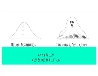
Normal Distribution: Fundamental Idea The normal (or Gaussian) distribution is perhaps the most famous continuous probability distribution. It is often used as the go-to distribution to represent the distribution of unknown random variables. Later in this course we will discuss the justification behind doing so. In the real-world, we might be trying to model measurement error, or the distribution of scores for an exam. These scenarios are naturally modeled by the normal distribution.

Definition For any µ ∈ R and σ > 0, a continuous random variable X with pdf 2 πσ 2 e − ( x − µ )2 1 f ( x ) = 2 σ 2 √ is called a normal random variable with mean parameter µ and variance σ 2 , and we write N ( µ, σ 2 ) In the special case where µ = 0 and σ = 1, X is a standard normal random variabe. The CDF of the standard normal has a special name, P ( X < x ) = Φ ( x ).

Picture

Check

Check f ( x ) is nonnegative. However, Z ∞ Z ∞ 2 πσ 2 e − ( x − µ )2 1 2 σ 2 dx = 1 f ( x ) dx = √ −∞ −∞ is true but tricky to verify (need to use polar coordinates).

Mean and Variance of Standard Normal

Mean and Variance of Standard Normal Z ∞ Z ∞ 1 e − x 2 2 dx = 0 E [ X ] = xf ( x ) dx = (1) x √ 2 π −∞ −∞ Var [ X ] = E [ X 2 ] − E [ X ] 2 = E [ X 2 ] (2) Z ∞ Z ∞ 1 e − x 2 x 2 f ( x ) dx = x 2 2 dx = 1 = (3) √ 2 π −∞ −∞

Scaling and Shifting Normals

Scaling and Shifting Normals If X ∼ N ( µ, σ 2 ), then Y = X − µ ∼ N (0 , 1). σ Proof: Let X ∼ N ( µ, σ 2 ), we can calculate the distribution of Y = X − µ σ P ( a ≤ Y ≤ b ) = P ( σ a + µ ≤ X ≤ σ b + µ ) (4) Z σ b + µ e − ( x − µ )2 1 2 σ 2 dx = (5) √ 2 πσ 2 σ a + µ Z b 1 e − y 2 2 dy = (6) √ 2 π a

Mean and Variance of Normal

Mean and Variance of Normal Let X ∼ N ( µ, σ 2 ), we know then that the distribution of Y = X − µ is N (0 , 1). σ So, ] = E [ X − µ ] 0 = E [ Y ] = E [ X − µ (7) σ σ ⇒ 0 = E [ X ] − µ (8) ⇒ E [ X ] = µ (9) For variance, ] = Var [ X − µ ] 1 = Var [ Y ] = Var [ X − µ (10) σ 2 σ ⇒ 1 = Var [ X ] (11) σ 2 ⇒ Var [ X ] = σ 2 (12)

What does this mean? We can relate any normal random variable X ∼ N ( µ, σ 2 ) to the standard normal Y : P ( X ≤ a ) = P ( Y ≤ a − µ ) = Φ ( a − µ ) σ σ Since the CDF uniquely characterizes a distribution, we use a table of precomputed values of Φ ( x ) to do computation with normal distributions.

Using Table of Precomputed Values If X ∼ N (60 , 20 2 ), and we want to find P ( X ≥ 80).

Using Table of Precomputed Values If X ∼ N (60 , 20 2 ), and we want to find P ( X ≥ 80). P ( X ≥ 80) = 1 − P ( X ≤ 80) . We can let Y = X − µ = X − 60 20 , so Y ∼ N (0 , 1). Then, σ P ( X ≤ 80) = P ( X − 60 ≤ 80 − 60 ) 20 20 = P ( Y ≤ 1) = Φ (1) = 0 . 8413 ... (using table) ⇒ P ( X ≥ 80) = 1 − 0 . 8413 ...

Standard Normal CDF Table

Nice Property: Sum of Indep. Gaussians is Gaussian If X ∼ N ( µ x , σ 2 x ) and Y ∼ N ( µ y , σ 2 y ), then Z = X + Y has distribution Z ∼ N ( µ x + µ y , σ 2 x + σ 2 y ) Proof: See notes/HW.

Two Envelopes Revisited Just like last time, one envelope contains x and the other contains 2 x , except this time you can look inside the envelope you are given and see how much money is inside before deciding to switch. Is there some strategy that can give you a better than 50% chance of getting the envelope with more money?

Two Envelopes Revisited