Why Gaussian and Cauchy Functions Computationally . . . Are - PowerPoint PPT Presentation

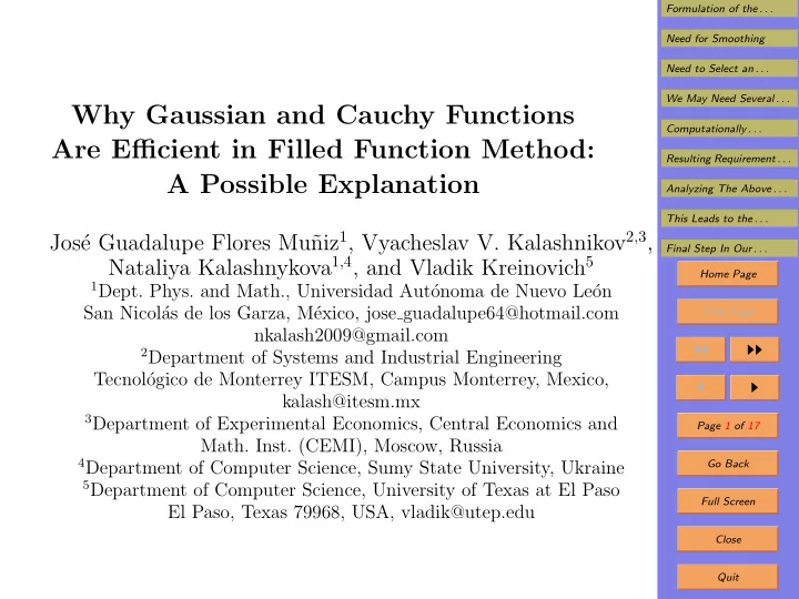
Formulation of the . . . Need for Smoothing Need to Select an . . . We May Need Several . . . Why Gaussian and Cauchy Functions Computationally . . . Are Efficient in Filled Function Method: Resulting Requirement . . . A Possible Explanation Analyzing The Above . . . This Leads to the . . . niz 1 , Vyacheslav V. Kalashnikov 2 , 3 , Jos´ e Guadalupe Flores Mu˜ Final Step In Our . . . Nataliya Kalashnykova 1 , 4 , and Vladik Kreinovich 5 Home Page 1 Dept. Phys. and Math., Universidad Aut´ onoma de Nuevo Le´ on San Nicol´ as de los Garza, M´ exico, jose guadalupe64@hotmail.com Title Page nkalash2009@gmail.com ◭◭ ◮◮ 2 Department of Systems and Industrial Engineering Tecnol´ ogico de Monterrey ITESM, Campus Monterrey, Mexico, ◭ ◮ kalash@itesm.mx 3 Department of Experimental Economics, Central Economics and Page 1 of 17 Math. Inst. (CEMI), Moscow, Russia 4 Department of Computer Science, Sumy State University, Ukraine Go Back 5 Department of Computer Science, University of Texas at El Paso Full Screen El Paso, Texas 79968, USA, vladik@utep.edu Close Quit

Formulation of the . . . Need for Smoothing 1. Outline Need to Select an . . . • One of the main problems of optimization algorithms We May Need Several . . . is that they end up in a local optimum. Computationally . . . Resulting Requirement . . . • It is necessary to get out of the local optimum and Analyzing The Above . . . eventually reach the global optimum. This Leads to the . . . • One of the promising methods to leave the local opti- Final Step In Our . . . mum is the filled function method. Home Page • Empirically, the best smoothing functions in this Title Page method are the Gaussian and the Cauchy functions. ◭◭ ◮◮ • In this talk, we provide a possible theoretical explana- ◭ ◮ tion for this empirical result. Page 2 of 17 Go Back Full Screen Close Quit

Formulation of the . . . Need for Smoothing 2. Formulation of the Problem Need to Select an . . . • Many optimization techniques end up in a local opti- We May Need Several . . . mum. Computationally . . . Resulting Requirement . . . • So, to solve a global optimization problem, it is neces- Analyzing The Above . . . sary to move out of the local minimum. This Leads to the . . . • Eventually, we should end up in a global minimum (or Final Step In Our . . . at least in a better local minimum). Home Page • One of the most efficient techniques for avoiding a local Title Page optimum is Renpu’s filled function method. ◭◭ ◮◮ • In this method, once we reach a local optimum x ∗ , we ◭ ◮ optimize an auxiliary expression Page 3 of 17 � x − x ∗ � · F ( f ( x ) , f ( x ∗ ) , x ) + G ( f ( x ) , f ( x ∗ ) , x ) , K Go Back σ Full Screen for some K, F, G, and σ. Close Quit

Formulation of the . . . Need for Smoothing 3. Formulation of the Problem (cont-d) Need to Select an . . . • We use its optimum as a new first approximation to We May Need Several . . . find the optimum of f ( x ). Computationally . . . Resulting Requirement . . . • Several different functions K ( x − x ∗ ) have been pro- Analyzing The Above . . . posed. This Leads to the . . . • It turns out that the most computationally efficient Final Step In Our . . . functions are the Gaussian and Cauchy functions Home Page 1 K ( x ) = exp( −� x � 2 ) , Title Page K ( x ) = 1 + � x � 2 . ◭◭ ◮◮ • Are these function indeed the most efficient? ◭ ◮ • Or they are simply the most efficient among a few func- Page 4 of 17 tions that have been tried? Go Back Full Screen Close Quit

Formulation of the . . . Need for Smoothing 4. What We Plan to Do Need to Select an . . . • In this talk, we formulate the above question as a pre- We May Need Several . . . cise mathematical problem. Computationally . . . Resulting Requirement . . . • We show that in this formulation, the Gaussian and the Analyzing The Above . . . Cauchy functions are indeed the most efficient ones. This Leads to the . . . • This result provides a possible theoretical explanation Final Step In Our . . . for the above empirical fact. Home Page • This results also shows that the Gaussian and the Title Page Cauchy functions K ( x ) are indeed the best. ◭◭ ◮◮ • This will hopefully make users more confident in (these ◭ ◮ versions of) the function filling method. Page 5 of 17 Go Back Full Screen Close Quit

Formulation of the . . . Need for Smoothing 5. Need for Smoothing Need to Select an . . . • One of the known ways to eliminate local optima is to We May Need Several . . . apply a weighted smoothing . Computationally . . . Resulting Requirement . . . • In this method, we replace the original objective func- Analyzing The Above . . . tion f ( x ) with a “smoothed” one This Leads to the . . . � x − x ′ � � def f ∗ ( x ) · f ( x ′ ) dx ′ , for some K ( x ) and σ. = Final Step In Our . . . K σ Home Page • The weighting function is usually selected in such a Title Page � way that K ( − x ) = K ( x ) and K ( x ) dx < + ∞ . ◭◭ ◮◮ ◭ ◮ • The first condition comes from the fact that we have no reason to prefer different orientations of coordinates. Page 6 of 17 Go Back • The second condition is that for f ( x ) = const, smooth- ing should leads to a finite constant. Full Screen Close Quit

Formulation of the . . . Need for Smoothing 6. Need to Select an Appropriate Value σ Need to Select an . . . • When σ is too small, the smoothing only covers a very We May Need Several . . . small neighborhood of each point x . Computationally . . . Resulting Requirement . . . • The smoothed function f ∗ ( x ) is close to the original Analyzing The Above . . . objective function f ( x ). This Leads to the . . . • So, we will still observe all the local optima. Final Step In Our . . . Home Page • On the other hand, if σ is too large, the smoothed function f ∗ ( x ) is too different from f ( x ). Title Page • So the optimum of the smoothed function may have ◭◭ ◮◮ nothing to do with the optimum of f ( x ). ◭ ◮ • So, for the smoothing method to work, it is important Page 7 of 17 to select an appropriate value of σ . Go Back Full Screen Close Quit

Formulation of the . . . Need for Smoothing 7. We May Need Several Iterations to Find an Need to Select an . . . Appropriate σ We May Need Several . . . • Our first estimate for σ may not be the best. Computationally . . . Resulting Requirement . . . • If we have smoothed the function too much, then we Analyzing The Above . . . need to “un-smooth” it, i.e., to select a smaller σ . This Leads to the . . . • If we have not smoothed the function enough, then we Final Step In Our . . . need to smooth it more, i.e., to select a larger σ . Home Page Title Page ◭◭ ◮◮ ◭ ◮ Page 8 of 17 Go Back Full Screen Close Quit

Formulation of the . . . Need for Smoothing 8. Computationally Efficient Smoothing: Analy- Need to Select an . . . sis We May Need Several . . . • Once we have smoothed the function too much, it is Computationally . . . difficult to un-smooth it. Resulting Requirement . . . Analyzing The Above . . . • Therefore, a usual approach is that we first try some small smoothing. This Leads to the . . . Final Step In Our . . . • If the resulting smoothed function f ∗ ( x ) still leads to a Home Page similar local maximum, we smooth it some more, etc. Title Page • For small σ : ◭◭ ◮◮ – to find each value f ∗ ( x ) of the smoothed function, ◭ ◮ – we only need to consider values of f ( x ′ ) in a small vicinity of x . Page 9 of 17 • The larger σ , the larger this vicinity, so: Go Back – the more values f ( x ′ ) we need to take into account, Full Screen – and thus the more computations we need. Close Quit

Formulation of the . . . Need for Smoothing 9. Computationally Efficient Smoothing: Conclu- Need to Select an . . . sion We May Need Several . . . • Let’s assume that we have a smoothed function f ∗ ( x ) Computationally . . . corresponding to some value of σ . Resulting Requirement . . . Analyzing The Above . . . • We need to compute a smoothed function f ∗∗ ( x ) cor- responding to a larger value σ ′ > σ . This Leads to the . . . Final Step In Our . . . • It is thus more computationally efficient not to apply Home Page smoothing with σ ′ to the original f ( x ). Title Page • Instead, we should apply a small additional smoothing ◭◭ ◮◮ to the smoothed function f ∗ ( x ). ◭ ◮ Page 10 of 17 Go Back Full Screen Close Quit

Formulation of the . . . Need for Smoothing 10. Resulting Requirement on the Smoothing Need to Select an . . . Function K ( x ) We May Need Several . . . • For every σ ′ and σ , there should be an appropriate Computationally . . . value ∆ σ . Resulting Requirement . . . Analyzing The Above . . . • Then, after we get This Leads to the . . . � x − x ′ � � f ∗ ( x ) = · f ( x ′ ) dx ′ . K Final Step In Our . . . σ Home Page • A smoothing with ∆ σ should lead to the desired func- Title Page tion ◭◭ ◮◮ � x − x ′ � � f ∗∗ ( x ) = · f ( x ′ ) dx ′ . K σ ′ ◭ ◮ • In other words, we need to make sure that for every Page 11 of 17 objective function f ( x ), we have Go Back � x − x ′ � x − x ′ � � � � · f ( x ′ ) dx ′ = · f ∗ ( x ′ ) dx ′ . Full Screen K K σ ′ ∆ σ Close Quit