Students t -Distribution The t -Distribution, t -Tests, & - PowerPoint PPT Presentation

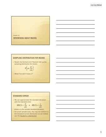
Student’s t -Distribution The t -Distribution, t -Tests, & Measures of Effect Size

Sampling Distributions Redux • Chapter 7 opens with a return to the concept of sampling distributions from chapter 4 – Sampling distributions of the mean

Sampling Distribution of the Mean • Because the SDotM is so important in statistics, you should understand it • The SDotM is governed by the Central Limit Theorem Given a population with a mean μ and a variance σ 2 , the sampling distribution of the mean (the distribution of sample means) will have a mean equal to μ , a variance equal to σ 2 /n, and a standard deviation equal to . The σ 2 / n distribution will approach the normal distribution as n, the sample size, increases. (p. 178)

Sampling Distribution of the Mean Translation: 1. For any population with a given mean and variance the sampling distribution of the mean will have: • μ x = μ 2 = σ 2 /n • σ x • σ x = σ / √ n 2. As n increases, the sampling distribution of the mean ( μ x ) approaches a normal curve

Sampling Distribution of the Mean • Analysis: – Although μ x and μ will tend to be similar to one another… – The relationships between… 2 and σ 2 • σ x • σ x and σ – …will differ as a function of the sample size • We saw this in our sampling distribution of the mean example from chapter 4…

So, you wanna test a hypothesis, do ya? • Our understanding of sampling and sampling distributions now allows us to test hypotheses • How we test a hypothesis depends on the information we have available

Choosing a Test • μ ? 1. Which variables are available? – σ ? – s? 2. How many data • Number of data sets: sets are you – 1 presented with? – 2 3. Do your data sets • Number of Groups come from 1 or 2 – 1 groups? – 2

Testing Hypotheses about Means: The Rare Case of Knowing σ − • So far, to test the ( x x ) = z σ probability of finding a − particular score, ( 83 100 ) = z 15 we’ve used the ( − 17 ) Standard Normal = z 15 Distribution = − z 1 . 3 3 – IQ = 83 – μ = 100 -1.96 < z < 1.96 Fail to reject H 0 – σ = 15

…The Rare Case of Knowing σ • Remember: we rarely know the population mean and standard deviation • This test can ONLY be used in situations where the population mean and standard deviation are known!

…The Rare Case of Knowing σ : • Stick with IQ: – μ = 100 – σ = 15 • However, we want to test a group of children against the population values for IQ – n = 5 (a group of 5 children)

…The Rare Case of Knowing σ : • Research Hypothesis: – The children’s IQ scores are different from the population IQ scores • H 1 : μ c ≠ μ p • Null Hypothesis – The children’s IQ scores do not differ from the population IQ scores • H 0 : μ c = μ p • Test the students (x-bar = 122)

…The Rare Case of Knowing σ : • Select: • Rejection region • α = .05 • “Tail” or directionality • We don’t know exactly how the students will score: we just expect them to show scores differing from the population values

…The Rare Case of Knowing σ : The z -Test • Generate sampling distribution of the mean assuming H 0 is true • z -Test • Given our sampling distribution: • Conduct the statistical test

Conducting the z -Test − μ ) Note: this equation is a modification of the ( x = original z -score formula z σ This formula adjusts z for sample size according to the rules of the central limit theorem n − ( 122 100 ) ( 22 ) ( 22 ) = = = = z 3 . 28 z z z 15 15 6 . 70 2 . 24 5 z = 3.28 > 1.96 : Reject H 0

How the z -Test Works n = 100 − ( 122 100 ) ( 22 ) ( 22 ) = = = = z 14 . 67 z z z 15 15 1 . 5 10 100 n = 2 − ( 122 100 ) ( 22 ) ( 22 ) = = = = z 2 . 07 z z z 15 15 10 . 64 1 . 41 2 − n = 1 ( 122 100 ) ( 22 ) ( 22 ) = = = = 1 . 47 z z z z 15 15 15 1 1

How the z -Test Works • Large samples reduce the amount of random variance (sampling error) – More confidence that the sample mean = population mean • Larger samples improve our ability to detect differences between samples and populations ( − μ ) • For n = 1 ( − μ ) x = x = z = z σ σ n

Statistical Tests We Have Learned 1. z -Test

Testing Hypotheses: When σ Is Unknown • Generally, the population standard deviation, σ , is unknown to us • Occasionally, we will know the population mean, μ , when we don’t know σ • In these situations, the standard normal distribution no longer meets our needs

Testing Hypotheses: When σ Is Unknown • Knowing μ … – We can produce an estimate of σ from s – Changes the nature of the test we are conducting, as s is not distributed in the same fashion as σ • Sampling distribution of the sample standard deviation is NOT normally distributed – Strong positive skew

Testing Hypotheses: When σ Is Unknown Sampling distribution of s Sampling distribution of σ

So How Does s Estimate σ ? • Given the differences in distribution shape, it is easy to conclude that s ≠ σ – s is an unbiased estimator of σ over repeated samplings – However, a SINGLE value of s is likely to underestimate σ • Because of this fact, small samples will systematically underestimate σ as a function of s – This leads to any given statistic calculated from this distribution to be < a comparable value of z – We cannot use z any longer � t

t and the t -Distribution • Developed by Student while he was working for the Guinness Brewing Co. 1. The shape of the t -distribution is a direct function of the size of the sample we are examining 2. For small samples, the t- distribution is somewhat flatter than the standard normal distribution, with a lower peak and fatter tails

t and the t -Distribution 3. As sample size increases: • The t- distribution approaches a normal distribution • Theoretically, we mean that the closer that our sample comes to infinity, the more it looks like a normal distribution • Practically, when n ~ 100 – 120

t and the t -Distribution

t and the t -Distribution 4. Identifying values of t associated with a given rejection region depends on: – α – the number of tails associated with the test – the degrees of freedom available in the analysis – For this one-sample test, (df = n-1) because we used one degree of freedom calculating s using the sample mean and not the population mean.

One-Sample t- Test − μ − μ − μ ( x ) ( x ) ( x ) = = = t t t s or or 2 s x s x x n n

z -Test vs. One-Sample t -Test ( − μ ) − μ x ( x ) = = z t σ s x n n Note the similarities between these tests: ONLY the source of “variance” and the distribution you test against have changed!

Using the One-Sample t -Test • You are one the admissions board for a graduate school of Psychology. • You are attempting to determine if the GRE scores for the students applying to your program is competitive with the national average. – μ Verbal = 569 – x-bar = 643 – s = 82 – n = 24

Using the One-Sample t -Test • Research Hypothesis: – The GRE scores from your applicants differ from the population norms • H 1 : μ a ≠ μ p • Null Hypothesis – The GRE scores from your applicants do not differ from the population norms • H 0 : μ a = μ p • Evaluate the students’ GRE-V scores

Using the One-Sample t -Test • Select: • Rejection region • α = .05 • “Tail” or directionality • We don’t know exactly how the students will score: we just expect them to show scores differing from the population values • Might predict higher scores…

Using the One-Sample t -Test • Generate sampling distribution of the mean assuming H 0 is true • One-Sample t -test • Given our sampling distribution: • Conduct the statistical test

Using the One-Sample t -Test − μ μ Verbal = ( x ) = t 569 s x-bar = x 643 n s = 82 n = 24 − ( 643 569 ) ( 74 ) ( 74 ) = = = = t 4 . 42 t t t 82 82 16 . 73 4 . 90 24 This numerical value is called t obt t obt (23) = 4.42

Evaluating Statistical Significance of the t -Test • First note: – α = .05 – Tail or directionality: two-tailed – t -Value = 4.42 – Degrees of freedom (df) • For the One-Sample t -Test, df = n-1 (24-1 = 23) • Estimating s from x-bar (not σ from μ )

p. 747 in Howell Text 1) Find row for TAIL 2) In the ROW for the correct tail, find α 3) Find df 4) Track ROW of df across to COLUMN of α The numerical value you obtain is called t crit t crit (23) = 2.069

Evaluating Statistical Significance of the t -Test • Compare t crit to our t obt value • If t obt falls into the rejection region identified by t crit , then we reject H 0 • If t obt does not fall into the rejection region identified by t crit , then we fail to reject H 0

Evaluating Statistical Significance of the t -Test t obt = 4.42 t crit = - 2.069 t crit = 2.069 0 Because t obt falls within the rejection region identified by t crit we reject H 0