Statistical Learning February 4, 2010 CS 489 / 698 University of - PowerPoint PPT Presentation
Statistical Learning February 4, 2010 CS 489 / 698 University of Waterloo Outline Statistical learning Bayesian learning Maximum a posteriori Maximum likelihood Learning from complete Data Reading: R&N Ch
Statistical Learning February 4, 2010 CS 489 / 698 University of Waterloo
Outline • Statistical learning – Bayesian learning – Maximum a posteriori – Maximum likelihood • Learning from complete Data • Reading: R&N Ch 20.1-20.2 2 CS489/698 Lecture Slides (c) 2010 P. Poupart
Statistical Learning • View: we have uncertain knowledge of the world • Idea: learning simply reduces this uncertainty 3 CS489/698 Lecture Slides (c) 2010 P. Poupart
Candy Example • Favorite candy sold in two flavors: – Lime (hugh) – Cherry (yum) • Same wrapper for both flavors • Sold in bags with different ratios: – 100% cherry – 75% cherry + 25% lime – 50% cherry + 50% lime – 25% cherry + 75% lime – 100% lime 4 CS489/698 Lecture Slides (c) 2010 P. Poupart
Candy Example • You bought a bag of candy but don’t know its flavor ratio • After eating k candies: – What’s the flavor ratio of the bag? – What will be the flavor of the next candy? 5 CS489/698 Lecture Slides (c) 2010 P. Poupart
Statistical Learning • Hypothesis H: probabilistic theory of the world – h 1 : 100% cherry – h 2 : 75% cherry + 25% lime – h 3 : 50% cherry + 50% lime – h 4 : 25% cherry + 75% lime – h 5 : 100% lime • Data D: evidence about the world – d 1 : 1 st candy is cherry – d 2 : 2 nd candy is lime – d 3 : 3 rd candy is lime – … 6 CS489/698 Lecture Slides (c) 2010 P. Poupart
Bayesian Learning • Prior: Pr(H) • Likelihood: Pr(d|H) • Evidence: d = <d 1 ,d 2 ,…,d n > • Bayesian Learning amounts to computing the posterior using Bayes’ Theorem: Pr(H| d ) = k Pr( d |H)Pr(H) 7 CS489/698 Lecture Slides (c) 2010 P. Poupart
Bayesian Prediction • Suppose we want to make a prediction about an unknown quantity X (i.e., the flavor of the next candy) • Pr(X| d ) = Σ i Pr(X| d ,h i )P(h i | d ) = Σ i Pr(X|h i )P(h i | d ) • Predictions are weighted averages of the predictions of the individual hypotheses • Hypotheses serve as “intermediaries” between raw data and prediction 8 CS489/698 Lecture Slides (c) 2010 P. Poupart
Candy Example • Assume prior P(H) = <0.1, 0.2, 0.4, 0.2, 0.1> • Assume candies are i.i.d. (identically and independently distributed) – P( d |h) = Π j P(d j |h) • Suppose first 10 candies all taste lime: – P( d |h 5 ) = 1 10 = 1 – P( d |h 3 ) = 0.5 10 = 0.00097 – P( d |h 1 ) = 0 10 = 0 9 CS489/698 Lecture Slides (c) 2010 P. Poupart
Posterior Posteriors given data generated from h_5 1 P(h_1|E) P(h_2|E) P(h_3|E) 0.8 P(h_4|E) P(h_i|e_1...e_t) P(h_5|E) 0.6 0.4 0.2 0 0 2 4 6 8 10 Number of samples 10 CS489/698 Lecture Slides (c) 2010 P. Poupart
Prediction Bayes predictions with data generated from h_5 Probability that next candy is lime 1 0.9 P(red|e_1...e_t) 0.8 0.7 0.6 0.5 0.4 0 2 4 6 8 10 Number of samples 11 CS489/698 Lecture Slides (c) 2010 P. Poupart
Bayesian Learning • Bayesian learning properties: – Optimal (i.e. given prior, no other prediction is correct more often than the Bayesian one) – No overfitting (prior can be used to penalize complex hypotheses) • There is a price to pay: – When hypothesis space is large Bayesian learning may be intractable – i.e. sum (or integral) over hypothesis often intractable • Solution: approximate Bayesian learning 12 CS489/698 Lecture Slides (c) 2010 P. Poupart
Maximum a posteriori (MAP) • Idea: make prediction based on most probable hypothesis h MAP – h MAP = argmax hi P(h i | d ) – P(X| d ) ≈ P(X|h MAP ) • In contrast, Bayesian learning makes prediction based on all hypotheses weighted by their probability 13 CS489/698 Lecture Slides (c) 2010 P. Poupart
Candy Example (MAP) • Prediction after – 1 lime: h MAP = h 3 , Pr(lime|h MAP ) = 0.5 – 2 limes: h MAP = h 4 , Pr(lime|h MAP ) = 0.75 – 3 limes: h MAP = h 5 , Pr(lime|h MAP ) = 1 – 4 limes: h MAP = h 5 , Pr(lime|h MAP ) = 1 – … • After only 3 limes, it correctly selects h 5 14 CS489/698 Lecture Slides (c) 2010 P. Poupart
Candy Example (MAP) • But what if correct hypothesis is h 4 ? – h 4 : P(lime) = 0.75 and P(cherry) = 0.25 • After 3 limes – MAP incorrectly predicts h 5 – MAP yields P(lime|h MAP ) = 1 – Bayesian learning yields P(lime| d ) = 0.8 15 CS489/698 Lecture Slides (c) 2010 P. Poupart
MAP properties • MAP prediction less accurate than Bayesian prediction since it relies only on one hypothesis h MAP • But MAP and Bayesian predictions converge as data increases • No overfitting (prior can be used to penalize complex hypotheses) • Finding h MAP may be intractable: – h MAP = argmax P(h| d ) – Optimization may be difficult 16 CS489/698 Lecture Slides (c) 2010 P. Poupart
MAP computation • Optimization: – h MAP = argmax h P(h| d ) = argmax h P(h) P( d |h) = argmax h P(h) Π i P(d i |h) • Product induces non-linear optimization • Take the log to linearize optimization – h MAP = argmax h log P(h) + Σ i log P(d i |h) 17 CS489/698 Lecture Slides (c) 2010 P. Poupart
Maximum Likelihood (ML) • Idea: simplify MAP by assuming uniform prior (i.e., P(h i ) = P(h j ) ∀ i,j) – h MAP = argmax h P(h) P( d |h) – h ML = argmax h P( d |h) • Make prediction based on h ML only: – P(X| d ) ≈ P(X|h ML ) 18 CS489/698 Lecture Slides (c) 2010 P. Poupart
Candy Example (ML) • Prediction after – 1 lime: h ML = h 5 , Pr(lime|h ML ) = 1 – 2 limes: h ML = h 5 , Pr(lime|h ML ) = 1 – … • Frequentist: “objective” prediction since it relies only on the data (i.e., no prior) • Bayesian: prediction based on data and uniform prior (since no prior ≡ uniform prior) 19 CS489/698 Lecture Slides (c) 2010 P. Poupart
ML properties • ML prediction less accurate than Bayesian and MAP predictions since it ignores prior info and relies only on one hypothesis h ML • But ML, MAP and Bayesian predictions converge as data increases • Subject to overfitting (no prior to penalize complex hypothesis that could exploit statistically insignificant data patterns) • Finding h ML is often easier than h MAP – h ML = argmax h Σ i log P(d i |h) 20 CS489/698 Lecture Slides (c) 2010 P. Poupart
Recommend
More recommend
Explore More Topics
Stay informed with curated content and fresh updates.
