LEARNING PROBABILISTIC MODELS AIMA CHAPTER 20 Instructor: Sael Lee - PowerPoint PPT Presentation

CSE 537 Fall 2015 LEARNING PROBABILISTIC MODELS AIMA CHAPTER 20 Instructor: Sael Lee Materials form AIMA resources, “Learning with Maximum Likelihood” by Andrew W. Moore and “The EM Algorithm: short tutorial” by S. Borman

OUTLINE Agents can handle uncertainty by using the methods of probability and decision theory, but first they must learn their probabilistic theories of the world from experience by formulating the learning task itself as a process of probabilistic inference.  Statistical learning  Bayesian learning  Learning with Complete data  Maximum-likelihood parameter learning  Learning with Hidden Variables: EM  General Form of EM  Unsupervised clustering: mixture of Gaussians  Learning Bayesian net with hidden variables  Learning HMM

STATISTICAL LEARNING  Bayesian view of learning:  Provides general solutions to the problems of noise, over-fitting and optimal prediction.   The data are evidence : instantiation of some or all of the random variables describing the domain.  The hypotheses are probabilistic theories of how the domain works, including logical theories as a special case.

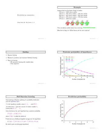
SURPRISE CANDY EXAMPLE Suppose there are five kinds of bags of candies: • 10% are h 1: 100% cherry candies • 20% are h 2: 75% cherry candies + 25% lime candies • 40% are h 3: 50% cherry candies + 50% lime candies • 20% are h 4: 25% cherry candies + 75% lime candies • 10% are h 5: 100% lime candies Given a new bag of candy, and we observe candies drawn from the bag: TASK1: What kind of bag is it? TASK2: What flavor will the next candy be?

POSTERIOR PROBABILITY OF HYPOTHESES TASK1: What kind of bag is it? Let hypothesis H={h1,..,h5} denote the type of the bag. Bayesian sian le learning Let D represent all the data with observed value d. Calculate the probability of each hypothesis given the data and predict on that basis. Probabilities of each hypothesis are obtained by Bayes’ rule. likelihood 10% are h 1: 100% cherry 20% are h 2: 75% cherry + 25% lime 40% are h 3: 50% cherry + 50% lime 20% are h 4: 25% cherry + 75% lime 10% are h 5: 100% lime Hypothesis posterior Probability of bag type given prior observations Likelihood of data under i.i.d. assumption 𝑄 ( ℎ 𝑗 )

PREDICTION PROBABILITY TASK2: What flavor will the next candy be? Prediction about an unknown quantity X, Predictions are weighted avg. over the predictions of the individual hypothesis. posterior Prediction Probability that next candy is lime given observations assuming that each hypothesis determines a probability distribution over X.

OPTIMALITY OF BAYESIAN PREDICTION  The Bayesian prediction eventually agrees with the true hypothesis  For any fixed prior that does not rule out the true hypothesis, the posterior probability of any fals e hypothesis will, under certain technical condit ions, eventually vanish.  Bayesian prediction is optimal whether the data se t be small or large. Given the hypothesis prior, a ny other prediction is expected to be correct less often.

REALITY  In real learning problems, the hypothesis space is usually very large or infinite Summing over the hypothesis space is often intractable (e.g., 18,446,744,073,709,551,616 Boolean functions of 6 attributes) Need approximation/simplified method for selecting the hypothesis

MAXIMUM A POSTERIORI (MAP) APPROXIMATION Make predictions based on a sin single mo most pr probable h hypo pothesis MAP learning chooses the hypothesis that provides maximum compression • of the data. log 2 P(h i ): the number of bits required to specify the hypothesis h i . • log 2 P(d d | h i ): the additional number of bits required to specify the data, • given the hypothesis.

MAP VS BAYESIAN EX> After three observations MAP predict with probability 1 that next candy is lime (pick h5) Bayes will predict with probability 0.8 that net is lime Probability that next candy is lime given observations

MAP & BAYESIAN – CONTROLLING COMPLEXITY ** BOTH MAP and Bayes penalize complexity using prior probability 𝑄 ( ℎ 𝑗 ) • High 𝑄 ( ℎ 𝑗 ) high penalty Typically, more comple lex hypothesis have a lower p prior probab abilit ity y – in part because there are casually many more complex hypothesis that simple hypotheses. On the other hand, more complex hypothesis save a greater capacity to fit the data.

MAXIMUM-LIKELIHOOD (ML) HYPOTHESIS APPROX. Assume uniform prior over the space of hypothesis MAP with uniform prior: Maximum-likelihood hypothesis Becomes irrelevant if uniform ML hypotheses is good for cases: Cannot trust the subjective nature of hypothesis prior • No reason to prefer one hypothesis over another • When complexity of each hypothesis is all similar • Good approximation when you have large dataset (problem if not) •

LEARNING WITH COMPLETE DATA The general task of learning a probability model, given data that are assumed to be generated form that model is called densit sity y estima matio ion. For simplicity, lets assume we have com complete d data, i.e., each data point contains values for every variable (feature) in the probability model being learned. – no missing data (fully observable) Parameter lea earni ning: Finding the numerical parameters for a probability model whose structure if fixed. Struc ucture lea earni ning: Finding the structure of the probability model.

ML PARAMETER LEARNING: DISCRETE VARIABLE Parameter ranging form [0 .. 1] Just one variable <- Likelihood of observed data Finding maximum log likelihood

 ML parameter learning step: Write down an expression for the likelihood of the 1. data as a function of parameters Write down the derivation of the log likelihood 2. w.r.t. each parameters Find the parameter values such that the derivatives 3. are zero Non-trivial in practice  Use iterative methods and/or numerical optimization  techniques Problem with ML  When the data set is small enough that some events  have not yet been observed, the ML hypothesis assigns zero probability to those events.

ML: MULTIPLE PARAMETERS N candies unwrapped, c are cherries and l are limes Take logarithm With complete data, the ML parameter learning problem for a Bayesian network decomposes into separate learning problems, one for each parameter

ML: MULTIPLE PARAMETERS CONT.

ML FOR CONTINUOUS MODELS  Example: Linear Gaussian model  Learning the parameters of a Gaussian density function on a single variable.  Data are generated as follows:  Let the observed values be x 1 , . . . , x N . Then the log likelihood is:  Setting the derivatives to zero as usual, we obtain

ML FOR CONTINUOUS MODELS EXAMPLE: LINEAR GAUSSIAN MODEL EX> One continuous parent X an a continuous child Y. Y has Gaussian distribution whose mean depends linearly on the value of X and whose std is fixed. X Y linear Gaussian model described as y = 𝛪 1 x + 𝛪 2 plus Gaussian noise with fixed variance. A set of 50 data points generated from this model That is, mi minimizing t the s sum m of squared er errors gives the ML solution for a linear fit assum ssuming ng Gaussi ussian n n noise o of fixed varianc nce

BAYESI SIAN P PARAMETER L LEARNING  Maximum-likelihood learning gives rise to some very simple procedures, but it has some serious deficiencies with small data sets  The Bayesian approach to parameter learning:  Starts by defining a prior probability distribution (hypothesis s pr prio ior) over the possible hypotheses.  Then, as data arrives, the posterior probability distribution is updated.