Learning in Graphical Models Marco Chiarandini Department of - PowerPoint PPT Presentation

Lecture 13 Learning in Graphical Models Marco Chiarandini Department of Mathematics & Computer Science University of Southern Denmark

Learning Graphical Models Course Overview Unsupervised Learning ✔ Introduction Learning ✔ Artificial Intelligence ✔ Supervised ✔ Intelligent Agents Decision Trees, Neural Networks ✔ Search Learning Bayesian Networks ✔ Uninformed Search ✔ Unsupervised ✔ Heuristic Search EM Algorithm ✔ Uncertain knowledge and Reinforcement Learning Reasoning Games and Adversarial Search ✔ Probability and Bayesian approach Minimax search and ✔ Bayesian Networks Alpha-beta pruning ✔ Hidden Markov Chains Multiagent search ✔ Kalman Filters Knowledge representation and Reasoning Propositional logic First order logic Inference Plannning 2

Learning Graphical Models Outline Unsupervised Learning 1. Learning Graphical Models Parameter Learning in Bayes Nets Bayesian Parameter Learning 2. Unsupervised Learning k-means EM Algorithm 3

Learning Graphical Models Outline Unsupervised Learning Methods: 1. Bayesian learning 2. Maximum a posteriori and maximum likelihood learning Bayesian networks learning with complete data a. ML parameter learning b. Bayesian parameter learning 4

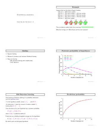
Learning Graphical Models Full Bayesian learning Unsupervised Learning View learning as Bayesian updating of a probability distribution over the hypothesis space H hypothesis variable, values h 1 , h 2 , . . . , prior Pr ( h ) d j gives the outcome of random variable D j (the j th observation) training data d = d 1 , . . . , d N Given the data so far, each hypothesis has a posterior probability: P ( h i | d ) = α P ( d | h i ) P ( h i ) where P ( d | h i ) is called the likelihood Predictions use a likelihood-weighted average over the hypotheses: � � Pr ( X | d ) = Pr ( X | d , h i ) P ( h i | d ) = Pr ( X | h i ) P ( h i | d ) i i Or predict according to the most probable hypothesis (maximum a posteriori) 5

Learning Graphical Models Example Unsupervised Learning Suppose there are five kinds of bags of candies: 10% are h 1 : 100% cherry candies 20% are h 2 : 75% cherry candies + 25% lime candies 40% are h 3 : 50% cherry candies + 50% lime candies 20% are h 4 : 25% cherry candies + 75% lime candies 10% are h 5 : 100% lime candies Then we observe candies drawn from some bag: What kind of bag is it? What flavour will the next candy be? 6

Learning Graphical Models Posterior probability of hypotheses Unsupervised Learning 1 P ( h 1 | d ) Posterior probability of hypothesis P ( h 2 | d ) P ( h 3 | d ) 0.8 P ( h 4 | d ) P ( h 5 | d ) 0.6 0.4 0.2 0 0 2 4 6 8 10 Number of samples in d 7

Learning Graphical Models Prediction probability Unsupervised Learning 1 0.9 P (next candy is lime | d ) 0.8 0.7 0.6 0.5 0.4 0 2 4 6 8 10 Number of samples in d 8

Learning Graphical Models MAP approximation Unsupervised Learning Summing over the hypothesis space is often intractable (e.g., 18,446,744,073,709,551,616 Boolean functions of 6 attributes) Maximum a posteriori (MAP) learning: choose h MAP maximizing P ( h i | d ) I.e., maximize P ( d | h i ) P ( h i ) or log P ( d | h i ) + log P ( h i ) Log terms can be viewed as (negative of) bits to encode data given hypothesis + bits to encode hypothesis This is the basic idea of minimum description length (MDL) learning For deterministic hypotheses, P ( d | h i ) is 1 if consistent, 0 otherwise = ⇒ MAP = simplest consistent hypothesis 9

Learning Graphical Models ML approximation Unsupervised Learning For large data sets, prior becomes irrelevant Maximum likelihood (ML) learning: choose h ML maximizing P ( d | h i ) I.e., simply get the best fit to the data; identical to MAP for uniform prior (which is reasonable if all hypotheses are of the same complexity) ML is the “standard” (non-Bayesian) statistical learning method 10

Learning Graphical Models Parameter learning by ML Unsupervised Learning ( ) Bag from a new manufacturer; fraction θ of cherry candies? P F=cherry θ Any θ is possible: continuum of hypotheses h θ θ is a parameter for this simple (binomial) family of models Flavor Suppose we unwrap N candies, c cherries and ℓ = N − c limes These are i.i.d. (independent, identically distributed) observations, so N P ( d j | h θ ) = θ c · ( 1 − θ ) ℓ � P ( d | h θ ) = j = 1 Maximize this w.r.t. θ —which is easier for the log-likelihood: N � L ( d | h θ ) = log P ( d | h θ ) = log P ( d j | h θ ) = c log θ + ℓ log ( 1 − θ ) j = 1 dL ( d | h θ ) c ℓ c + ℓ = c c = θ − 1 − θ = 0 = ⇒ θ = d θ N Seems sensible, but causes problems with 0 counts! 12

Learning Graphical Models Multiple parameters Unsupervised Learning ( ) P F=cherry Red/green wrapper depends probabilistically on flavor: θ Likelihood for, e.g., cherry candy in green wrapper: Flavor P ( F = cherry , W = green | h θ,θ 1 ,θ 2 ) = P ( F = cherry | h θ,θ 1 ,θ 2 ) P ( W = green | F = cherry P ( W=red | F ) F θ = θ · ( 1 − θ 1 ) cherry 1 θ lime 2 Wrapper N candies, r c red-wrapped cherry candies, etc.: θ c ( 1 − θ ) ℓ · θ r c 1 ( 1 − θ 1 ) g c · θ r ℓ 2 ( 1 − θ 2 ) g ℓ P ( d | h θ,θ 1 ,θ 2 ) = [ c log θ + ℓ log ( 1 − θ )] L = + [ r c log θ 1 + g c log ( 1 − θ 1 )] + [ r ℓ log θ 2 + g ℓ log ( 1 − θ 2 )] 13

Learning Graphical Models Multiple parameters contd. Unsupervised Learning Derivatives of L contain only the relevant parameter: ∂ L c ℓ c = θ − 1 − θ = 0 = ⇒ θ = ∂θ c + ℓ ∂ L r c g c r c = − = 0 = ⇒ θ 1 = ∂θ 1 θ 1 1 − θ 1 r c + g c ∂ L r ℓ g ℓ r ℓ = − = 0 = ⇒ θ 2 = ∂θ 2 θ 2 1 − θ 2 r ℓ + g ℓ With complete data, parameters can be learned separately 14

Learning Graphical Models Continuous models Unsupervised Learning 1 exp − ( x − µ ) 2 P ( x ) = √ 2 σ 2 2 πσ Parameters µ and σ 2 Maximum likelihood: 15

Learning Graphical Models Continuous models, Multiple param. Unsupervised Learning 1 0.8 P ( y | x ) 4 0.6 3.5 3 y 2.5 0.4 2 1.5 1 0 0.20.40.60.81 0.2 0.5 0 0 0.2 y 0.4 0.6 0 0.8 1 x 0 0.1 0.2 0.3 0.4 0.5 0.6 0.7 0.8 0.9 1 x 1 e − ( y − ( θ 1 x + θ 2 )) 2 √ Maximizing P ( y | x ) = 2 σ 2 w.r.t. θ 1 , θ 2 2 πσ N � ( y j − ( θ 1 x j + θ 2 )) 2 = minimizing E = j = 1 That is, minimizing the sum of squared errors gives the ML solution for a linear fit assuming Gaussian noise of fixed variance 16

Learning Graphical Models Summary Unsupervised Learning Full Bayesian learning gives best possible predictions but is intractable MAP learning balances complexity with accuracy on training data Maximum likelihood assumes uniform prior, OK for large data sets 1. Choose a parameterized family of models to describe the data requires substantial insight and sometimes new models 2. Write down the likelihood of the data as a function of the parameters may require summing over hidden variables, i.e., inference 3. Write down the derivative of the log likelihood w.r.t. each parameter 4. Find the parameter values such that the derivatives are zero may be hard/impossible; gradient techniques help 17

Learning Graphical Models Bayesian Parameter Learning Unsupervised Learning If small data set the ML method leads to premature conclusions: From the Flavor example: N c P ( d j | h θ ) = θ c · ( 1 − θ ) ℓ � P ( d | h θ ) = = ⇒ θ = c + ℓ j = 1 If N = 1 and c = 1, l = 0 we conclude θ = 1. Laplace adjustment can mitigate this result but it is artificial. 19

Learning Graphical Models Unsupervised Learning Bayesian approach: P ( θ | d ) = α P ( d | θ ) P ( θ ) we saw the likelihood to be p ( X = 1 | θ ) = Bern ( θ ) = θ which is known as Bernoulli distribution. Further, for a set of n observed outcomes d = ( x 1 , . . . , x n ) of which s are 1s, we have the binomial sampling model : � n � θ s ( 1 − θ ) n − s p ( D = d | θ ) = p ( s | θ ) = Bin ( s | θ ) = (1) s 20

Learning Graphical Models The Beta Distribution Unsupervised Learning We define the prior probability p ( θ ) to be Beta distributed p ( θ ) = Beta ( θ | a , b ) = Γ( a + b ) Γ( a )Γ( b ) θ a − 1 ( 1 − θ ) b − 1 2.5 6 [5,5] 5 [30,10] 2 [2,2] 4 P ( Θ = θ ) P ( Θ = θ ) 1.5 3 [1,1] 1 2 [6,2] 0.5 1 [3,1] 0 0 0 0.2 0.4 0.6 0.8 1 0 0.2 0.4 0.6 0.8 1 Parameter θ Parameter θ Reasons for this choice: provides flexiblity varying the hyperparameters a and b Eg. the uniform distribution is included in this family with a = 1, b = 1 conjugancy property 21

Learning Graphical Models Unsupervised Learning Eg: we observe N = 1, c = 1, l = 0: p ( θ | d ) = α p ( d | θ ) p ( θ ) = α Bin ( d | θ ) p ( θ ) = α Beta ( θ | a + c , b + l ) . 22