Probabilistic Graphical Models 10-708 Learning Partially Observed - - PDF document

SLIDE 1

1

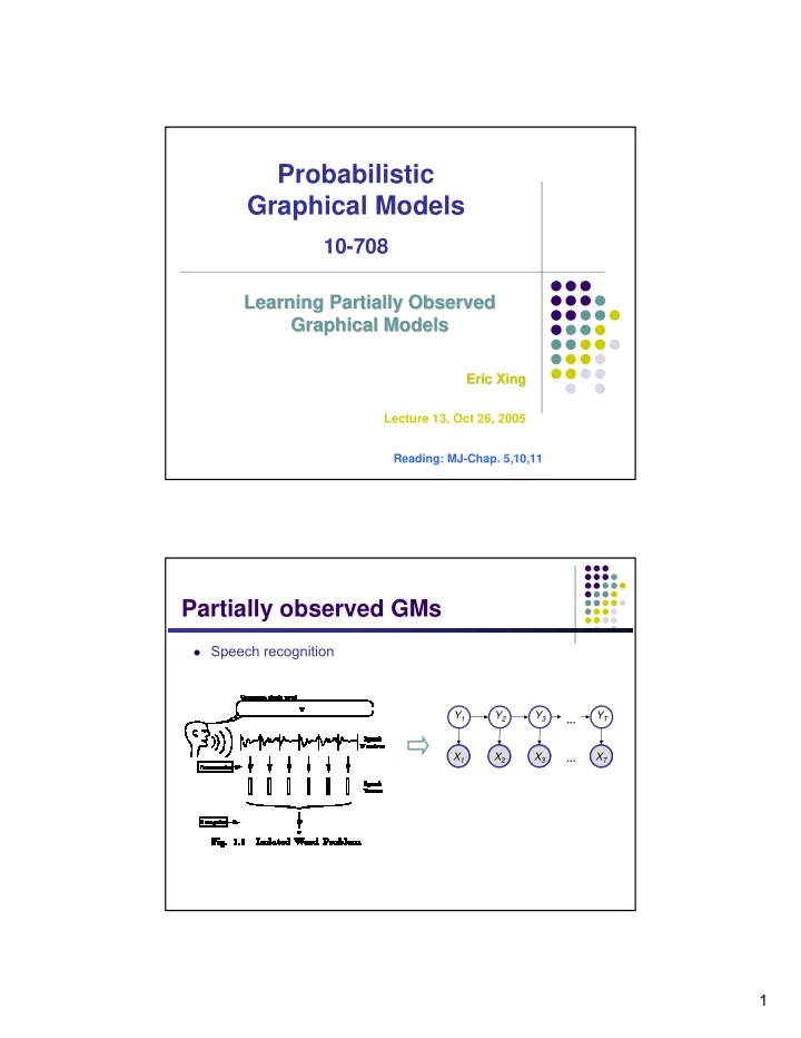
Probabilistic Graphical Models

10-708

Learning Partially Observed Learning Partially Observed Graphical Models Graphical Models

Eric Xing Eric Xing

Lecture 13, Oct 26, 2005 Reading: MJ-Chap. 5,10,11

Partially observed GMs

Speech recognition

A A A A

X2 X3 X1 XT Y2 Y3 Y1 YT

... ...

SLIDE 2

2

Partially observed GM

Biological Evolution

ancestor A C

Qh Qm

T years

?

A G A G A C

Unobserved Variables

A variable can be unobserved (latent) because:

• it is an imaginary quantity meant to provide some simplified and

abstractive view of the data generation process

• e.g., speech recognition models, mixture models …
• it is a real-world object and/or phenomena, but difficult or impossible to

measure

• e.g., the temperature of a star, causes of a disease, evolutionary

ancestors …

• it is a real-world object and/or phenomena, but sometimes wasn’t

measured, because of faulty sensors, etc.

Discrete latent variables can be used to partition/cluster data

into sub-groups.

Continuous latent variables (factors) can be used for

dimensionality reduction (factor analysis, etc).

SLIDE 3

3

Mixture models

A density model p(x) may be multi-modal. We may be able to model it as a mixture of uni-modal

distributions (e.g., Gaussians).

Each mode may correspond to a different sub-population

(e.g., male and female).

Gaussian Mixture Models (GMMs)

Consider a mixture of K Gaussian components:

• Z is a latent class indicator vector:
• X is a conditional Gaussian variable with a class-specific mean/covariance
• The likelihood of a sample:
• This model can be used for unsupervised clustering.
• This model (fit by AutoClass) has been used to discover new kinds of stars in

astronomical data, etc.

( )

∏

) : ( multi ) (

k z k n n

k n

z z p π π = =

{ }

)

• (

)

• (
• exp

) ( ) , , | (

/ / k n k T k n k m k n n

x x z x p µ µ π µ

1 2 1 2 1 2

2 1 1

−

Σ Σ = Σ = ( )

( ) ∑

∑ ∏ ∑

Σ = Σ = Σ = = = Σ

k k k k z k z k k n z k k k k n

x N x N z x p z p x p

n k n k n

) , | , ( ) , : ( ) , , | , ( ) | ( ) , ( µ π µ π µ π µ 1 1

mixture proportion mixture component

Z X

SLIDE 4

4

Conditional mixture model: Mixture of experts

• We will model p(Y |X) using different experts, each responsible for

different regions of the input space.

• Latent variable Z chooses expert using softmax gating function:
• Each expert can be a linear regression model:
• The posterior expert responsibilities are

( )

x x z P

T k

ξ Softmax ) ( = = 1

( )

2

1

k T k k

x y z x y P σ θ , ; ) , ( N = =

∑

= = = =

j j j j j k k k k k

x y p x z p x y p x z p y x z P ) , , ( ) ( ) , , ( ) ( ) , , (

2 2

1 1 1 σ θ σ θ θ

Hierarchical mixture of experts

• This is like a soft version of a depth-2 classification/regression tree.
• P(Y |X,G1,G2) can be modeled as a GLIM, with parameters

dependent on the values of G1 and G2 (which specify a "conditional path" to a given leaf in the tree).

SLIDE 5

5

Mixture of overlapping experts

By removing the X Z arc, we can make the partitions

independent of the input, thus allowing overlap.

This is a mixture of linear regressors; each subpopulation has

a different conditional mean.

∑

= = = =

j j j j j k k k k k

x y p z p x y p z p y x z P ) , , ( ) ( ) , , ( ) ( ) , , (

2 2

1 1 1 σ θ σ θ θ

Why is Learning Harder?

In fully observed iid settings, the log likelihood decomposes

into a sum of local terms (at least for directed models).

With latent variables, all the parameters become coupled

together via marginalization ) , | ( log ) | ( log ) | , ( log ) ; (

x z c

z x p z p z x p D θ θ θ θ + = = l

∑ ∑

= =

z x z z c

z x p z p z x p D ) , | ( ) | ( log ) | , ( log ) ; ( θ θ θ θ l

SLIDE 6

6

Gradient Learning for mixture models

We can learn mixture densities using gradient descent on the

log likelihood. The gradients are quite interesting:

In other words, the gradient is the responsibility weighted sum

• f the individual log likelihood gradients.

Can pass this to a conjugate gradient routine.

∑ ∑ ∑ ∑ ∑

∂ ∂ = ∂ ∂ = ∂ ∂ = ∂ ∂ = ∂ ∂ = =

k k k k k k k k k k k k k k k k k k k k k k k k k

r p p p p p p p p p p θ θ θ θ θ π θ θ θ θ π θ θ π θ θ θ π θ θ l l l ) x ( log ) | x ( ) x ( ) x ( log ) x ( ) | x ( ) x ( ) | x ( ) x ( log ) | x ( log ) ( 1

Parameter Constraints

Often we have constraints on the parameters, e.g. Σkπk = 1, Σ

being symmetric positive definite (hence Σii > 0).

We can use constrained optimization, or we can

reparameterize in terms of unconstrained values.

• For normalized weights, use the softmax transform:
• For covariance matrices, use the Cholesky decomposition:

where A is upper diagonal with positive diagonal: the parameters γi, λi, ηij ∈ R are unconstrained.

• Use chain rule to compute

) exp( ) exp(

j j k

k γ γ

π

Σ

= A A

T

= Σ−1

( )

) ( ) ( exp i j i j

ij ij ij i ii

< = > = > = A A A η λ

. , A ∂ ∂ ∂ ∂ l l π

SLIDE 7

7

Identifiability

A mixture model induces a multi-modal likelihood. Hence gradient ascent can only find a local maximum. Mixture models are unidentifiable, since we can always switch

the hidden labels without affecting the likelihood.

Hence we should be careful in trying to interpret the

“meaning” of latent variables.

Expectation-Maximization (EM) Algorithm

EM is an optimization strategy for objective functions that can

be interpreted as likelihoods in the presence of missing data.

It is much simpler than gradient methods:

• No need to choose step size.
• Enforces constraints automatically.
• Calls inference and fully observed learning as subroutines.

EM is an Iterative algorithm with two linked steps:

• E-step: fill-in hidden values using inference, p(z|x, θt).
• M-step: update parameters t+1 using standard MLE/MAP method

applied to completed data

We will prove that this procedure monotonically improves (or

leaves it unchanged). Thus it always converges to a local

• ptimum of the likelihood.

SLIDE 8

8

Complete & Incomplete Log Likelihoods

Complete log likelihood

Let X denote the observable variable(s), and Z denote the latent variable(s). If Z could be observed, then

• Usually, optimizing lc() given both z and x is straightforward (c.f. MLE for fully
• bserved models).
• Recalled that in this case the objective for, e.g., MLE, decomposes into a sum of

factors, the parameter for each factor can be estimated separately.

• But given that Z is not observed, lc() is a random quantity, cannot be

maximized directly. Incomplete log likelihood

With z unobserved, our objective becomes the log of a marginal probability:

• This objective won't decouple

) | , ( log ) , ; (

def

θ θ z x p z x

c

= l

∑

= =

z c

z x p x p x ) | , ( log ) | ( log ) ; ( θ θ θ l

Expected Complete Log Likelihood

For any distribution q(z), define expected complete log likelihood:

• A deterministic function of θ
• Linear in lc() --- inherit its factorizabiility
• Does maximizing this surrogate yield a maximizer of the likelihood?

Jensen’s inequality

∑

=

z q c

z x p x z q z x ) | , ( log ) , | ( ) , ; (

def

θ θ θ l

∑ ∑ ∑

= = = =

z z z

x z q z x p x z q x z q z x p x z q z x p x p x ) | ( ) | , ( log ) | ( ) | ( ) | , ( ) | ( log ) | , ( log ) | ( log ) ; ( θ θ θ θ θ l

q q c

H z x x + ≥ ⇒ ) , ; ( ) ; ( θ θ l l

SLIDE 9

9

Lower Bounds and Free Energy

For fixed data x, define a functional called the free energy: The EM algorithm is coordinate-ascent on F :

• E-step:
• M-step:

) ; ( ) | ( ) | , ( log ) | ( ) , (

def

x x z q z x p x z q q F

z

θ θ θ l ≤ = ∑ ) , ( max arg

t q t

q F q θ =

+1

) , ( max arg

t t t

q F θ θ

θ 1 1 + + =

E-step: maximization of expected lc w.r.t. q

Claim:

• This is the posterior distribution over the latent variables given the data

and the parameters. Often we need this at test time anyway (e.g. to perform classification).

Proof (easy): this setting attains the bound l(θ;x)≥F(q,θ ) Can also show this result using variational calculus or the fact

that

) , | ( ) , ( max arg

t t q t

x z p q F q θ θ = =

+1

) ; ( ) | ( log ) | ( log ) | ( ) , ( ) | , ( log ) , ( ) ), , ( ( x x p x p x z q x z p z x p x z p x z p F

t t z t z t t t t t

θ θ θ θ θ θ θ θ l = = = =

∑ ∑

( )

) , | ( || KL ) , ( ) ; ( θ θ θ x z p q q F x = − l

SLIDE 10

10

E-step ≡ plug in posterior expectation of latent variables

Without loss of generality: assume that p(x,z|θ) is a

generalized exponential family distribution:

• Special cases: if p(X|Z) are GLIMs, then

The expected complete log likelihood under

is

) ( ) , ( ) ( ) | , ( log ) , | ( ) , ; (

) , | (

θ θ θ θ θ θ

θ

A z x f A z x p x z q z x

i x z q i t i z t t q t c

t t

− = − =

∑ ∑

+1

l ⎭ ⎬ ⎫ ⎩ ⎨ ⎧ =

∑

i i i

z x f z x h Z z x p ) , ( exp ) , ( ) ( ) , ( θ θ θ 1

) ( ) ( ) , ( x z z x f

i T i i

ξ η =

) , | (

t t

x z p q θ =

+1

) ( ) ( ) (

) , | ( GLIM ~

θ ξ η θ

θ

A x z

i i x z q i t i p

t

− = ∑

M-step: maximization of expected lc w.r.t. θ

Note that the free energy breaks into two terms:

• The first term is the expected complete log likelihood (energy) and the

second term, which does not depend on θ, is the entropy.

Thus, in the M-step, maximizing with respect to θ for fixed q

we only need to consider the first term:

• Under optimal qt+1, this is equivalent to solving a standard MLE of fully
• bserved model p(x,z|θ), with the sufficient statistics involving z

replaced by their expectations w.r.t. p(z|x,θ).

q q c z z z

H z x x z q x z q z x p x z q x z q z x p x z q q F + = − = =

∑ ∑ ∑

) , ; ( ) | ( log ) | ( ) | , ( log ) | ( ) | ( ) | , ( log ) | ( ) , ( θ θ θ θ l

∑

= =

+

+ z q c t

z x p x z q z x

t

) | , ( log ) | ( max arg ) , ; ( max arg θ θ θ

θ θ

1

1

l

SLIDE 11

11

EM Constructs Sequential Convex Lower Bounds

Consider the likelihood function and the function F(qt+1, ·). A hill-climbing algorithm

Summary: EM Algorithm

• A way of maximizing likelihood function for latent variable
• models. Finds MLE of parameters when the original (hard)

problem can be broken up into two (easy) pieces:

1.

Estimate some “missing” or “unobserved” data from observed data and current parameters.

2.

Using this “complete” data, find the maximum likelihood parameter estimates.

• Alternate between filling in the latent variables using the best

guess (posterior) and updating the parameters based on this guess:

• E-step:
• M-step:
• In the M-step we optimize a lower bound on the likelihood. In

the E-step we close the gap, making bound=likelihood.

) , ( max arg

t q t

q F q θ =

+1

) , ( max arg

t t t

q F θ θ

θ 1 1 + + =

SLIDE 12

12

Example: Gaussian mixture model

A mixture of K Gaussians:

• Z is a latent class indicator vector
• X is a conditional Gaussian variable with a class-specific mean/covariance
• The likelihood of a sample:

The expected complete log likelihood

GM:

Zn Xn

N

( )

∏

) : ( multi ) (

k z k n n

k n

z z p π π = =

{ }

)

• (

)

• (
• exp

) ( ) , , | (

/ / k n k T k n k m k n n

x x z x p µ µ π µ

1 2 1 2 1 2

2 1 1

−

Σ Σ = Σ =

( )

( ) ∑

∑ ∏ ∑

Σ = Σ = Σ = = = Σ

k k k k z k z k k n z k k k k n

x N x N z x p z p x p

n k n k n

) , | , ( ) , : ( ) , , | , ( ) | ( ) , ( µ π µ π µ π µ 1 1

( )

∑ ∑ ∑ ∑ ∑ ∑

log ) ( ) ( 2 1 log ) , , | ( log ) | ( log ) , ; (

) | ( ) | ( n k k k n k T k n k n n k k k n n x z p n n n x z p n c

C x x z z z x p z p z x + Σ + − Σ − − = Σ + =

−

µ µ π µ π

1

θ l

We maximize iteratively using the following

iterative procedure:

─ Expectation step: computing the expected value of the hidden variables (i.e., z) given current est. of the parameters (i.e., π and µ).

• Here we are essentially doing inference

∑

) , | , ( ) , | , ( ) , , | (

) ( ) ( ) ( ) ( ) ( ) ( ) ( ) ( ) (

) (

i t i t i n t i t k t k n t k t t k n q k n t k n

x N x N x z p z

t

Σ Σ = Σ = = = µ π µ π µ τ 1

) (θ

c

l

E-step

Zn Xn

N

SLIDE 13

13

We maximize iteratively using the following

iterative procudure:

─ Maximization step: compute the parameters under current results of the expected value of the hidden variables

• This is isomorphic to MLE except that the variables that are hidden are

replaced by their expectations (in general they will by replaced by their corresponding "sufficient statistics")

) (θ

c

l

M-step

Zn Xn

N

⇒ s.t. , ∀ , ) ( ⇒ , ) ( max arg

) ( * k ∂ ∂ *

∑ ∑

) (

N n N N z k l l

k n t k n n q k n k k c c k

t k

= = = = = =

∑ τ

π π π

π

1 θ θ

∑ ∑

) ( ) ( ) ( *

⇒ , ) ( max arg

n t k n n n t k n t k k

x l τ τ µ µ = =

+1

θ

∑ ∑

) ( ) ( ) ( ) ( ) ( *

) )( ( ⇒ , ) ( max arg

n t k n n T t k n t k n t k n t k k

x x l τ µ µ τ

1 1 1 + + +

− − = Σ = Σ θ

T T T

xx x x = ∂ ∂ = ∂ ∂

− −

A A A A A log : Fact

1 1

EM for MOG

SLIDE 14

14

Compare: K-means

The EM algorithm for mixtures of Gaussians is like a "soft

version" of the K-means algorithm.

In the K-means “E-step” we do hard assignment: In the K-means “M-step” we update the means as the

weighted sum of the data, but now the weights are 0 or 1: ) ( ) ( max arg

) ( ) ( ) ( ) ( t k n t k T t k n k t n

x x z µ µ − Σ − =

−1

∑ ∑

=

+ n t n n n t n t k

k z x k z ) , ( ) , (

) ( ) ( ) (

δ δ µ

1

EM for conditional mixture model

Model: The objective function EM:

• E-step:
• M-step:
• using the normal equation for standard LR

, but with the data re-weighted by τ (homework)

• IRLS and/or weighted IRLS algorithm to update {ξk, θk, σk} based on data pair

(xn,yn), with weights (homework)

) , , , | ( ) , | ( ) ( σ θ ξ

i k k k

x z y p x z p x y P 1 1 = = =∑

∑

= = = = =

j j j n n j n j n k k n n k n k n n n k n t k n

x y p x z p x y p x z p y x z P ) , , ( ) ( ) , , ( ) ( ) , , (

) ( 2 2

1 1 1 σ θ σ θ τ θ

( )

∑ ∑ ∑ ∑ ∑ ∑

log )

• (

2 1 ) softmax( log ) , , , | ( log ) , | ( log ) , , ; (

) , | ( ) , | ( n k k k n T k n k n n k n T k k n n y x z p n n n n y x z p n n c

C x y z x z z x y p x z p z y x ⎟ ⎟ ⎠ ⎞ ⎜ ⎜ ⎝ ⎛ + + − = + =

2 2

σ σ θ ξ σ θ ξ θ l

Y X X X

T T 1 −

= ) ( θ

) (t k n

τ

SLIDE 15

15

EM for general BNs

while not converged % E-step for each node i ESSi = 0 % reset expected sufficient statistics for each data sample n do inference with Xn,H for each node i % M-step for each node i θi := MLE(ESSi )

) | ( , ,

, ,

) , (

H n H n i

x x p n i n i i

x x SS ESS

−

= +

π

Partially Hidden Data

Of course, we can learn when there are missing (hidden)

variables on some cases and not on others.

In this case the cost function is:

• Note that Ym do not have to be the same in each case --- the data can

have different missing values in each different sample

Now you can think of this in a new way: in the E-step we

estimate the hidden variables on the incomplete cases only.

The M-step optimizes the log likelihood on the complete data

plus the expected likelihood on the incomplete data using the E-step.

∑ ∑ ∑

∈ ∈

+ =

Missing Complete

) | , ( log ) | , ( log ) ; (

m y m m n n n c

m

y x p y x p D θ θ θ l

SLIDE 16

16

EM Variants

Sparse EM:

Do not re-compute exactly the posterior probability on each data point under all models, because it is almost zero. Instead keep an “active list” which you update every once in a while.

Generalized (Incomplete) EM:

It might be hard to find the ML parameters in the M-step, even given the completed data. We can still make progress by doing an M-step that improves the likelihood a bit (e.g. gradient step). Recall the IRLS step in the mixture of experts model

A Report Card for EM

Some good things about EM:

• no learning rate (step-size) parameter
• automatically enforces parameter constraints
• very fast for low dimensions
• each iteration guaranteed to improve likelihood

Some bad things about EM:

• can get stuck in local minima
• can be slower than conjugate gradient (especially near convergence)
• requires expensive inference step
• is a maximum likelihood/MAP method