Lecture 22 & 23: Variational Autoencoders April 2020 Lecturer: - PDF document
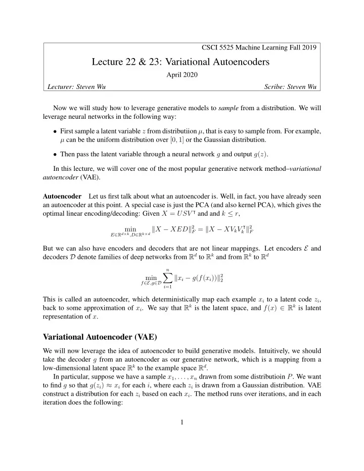
CSCI 5525 Machine Learning Fall 2019 Lecture 22 & 23: Variational Autoencoders April 2020 Lecturer: Steven Wu Scribe: Steven Wu Now we will study how to leverage generative models to sample from a distribution. We will leverage neural
CSCI 5525 Machine Learning Fall 2019 Lecture 22 & 23: Variational Autoencoders April 2020 Lecturer: Steven Wu Scribe: Steven Wu Now we will study how to leverage generative models to sample from a distribution. We will leverage neural networks in the following way: • First sample a latent variable z from distributiion µ , that is easy to sample from. For example, µ can be the uniform distribution over [0 , 1] or the Gaussian distribution. • Then pass the latent variable through a neural network g and output g ( z ) . In this lecture, we will cover one of the most popular generative network method– variational autoencoder (VAE). Autoencoder Let us first talk about what an autoencoder is. Well, in fact, you have already seen an autoencoder at this point. A special case is just the PCA (and also kernel PCA), which gives the optimal linear encoding/decoding: Given X = USV ⊺ and and k ≤ r , E ∈ R d × k ,D ∈ R k × d � X − XED � 2 k � 2 F = � X − XV k V ⊺ min F But we can also have encoders and decoders that are not linear mappings. Let encoders E and decoders D denote families of deep networks from R d to R k and from R k to R d n � � x i − g ( f ( x i )) � 2 min 2 f ∈E ,g ∈D i =1 This is called an autoencoder, which deterministically map each example x i to a latent code z i , back to some approximation of x i . We say that R k is the latent space, and f ( x ) ∈ R k is latent representation of x . Variational Autoencoder (VAE) We will now leverage the idea of autoencoder to build generative models. Intuitively, we should take the decoder g from an autoencoder as our generative network, which is a mapping from a low-dimensional latent space R k to the example space R d . In particular, suppose we have a sample x 1 , . . . , x n drawn from some distributioin P . We want to find g so that g ( z i ) ≈ x i for each i , where each z i is drawn from a Gaussian distribution. VAE construct a distribution for each z i based on each x i . The method runs over iterations, and in each iteration does the following: 1
1. Encode each example into Gaussian mean-variance parameters ( µ i , Σ i ) ← f ( x i ) . 2. Sample latent variable from Gaussian: z i ∼ N ( µ i , Σ i ) . 3. Decode ˆ x i = g ( z i ) . 4. Taking a gradient descent step (or any other optimization method) to further minimize the VAE objective n � � � N ( µ i , σ 2 ℓ ( x i , ˆ x i ) + λ KL i I ) , N (0 , I ) i =1 x i � 2 where ℓ ( x i , ˆ x i ) is “reconstruction error”. For example, ℓ ( x i , ˆ x i ) = � x i − ˆ 2 . We will go into the details of the gradient update step in a bit. In the VAE objective, KL denotes KL divergence: for any two distributions p and q , � p ( z ) ln p ( z ) KL ( p || q ) = q ( z ) dz KL divergence is a dissimilarity measure between distributions, with two important properties: • KL ( p || q ) ≥ 0 for any p, q . • KL ( p || q ) = KL ( q || p ) if and only if p = q . KL divergence encourages the individual distributions N ( µ i , Σ i ) to be close to the distribution N (0 , I ) . This is useful because N (0 , I ) is the “source” distribution for the generative models–that is, we output g ( z ) with z ∼ N (0 , I ) . The smaller the KL divergence is, the closer this sampling has to approximate the training distribution. Derivation from Variational Inference VAE is based on ideas from variatioinal inference (VI), which is a popular method to perform approximate inference in probabilistic models. We won’t get into the details of VI here, but we will discuss the relevant ideas that lead to VAE. Let P = { p θ | θ ∈ Θ } be a family of probability distributions over observed and latent variables x and z . Given a set of observed variables S = { x 1 , . . . , x n } , we would like to find a distribution in P to minimize: p S ( x ) ln ˆ p S ( x ) � p S || p ) = min min p ∈P KL (ˆ ˆ p ( x ) p ∈P x ∈ S p S denotes the empirical distribution over the data set. Note that � where ˆ x ∈ S ˆ p s ( x ) ln p s ( x ) does not depend on the choice of p . Thus, the minimization is equivalent to the following maximization problem: � � � � max p S ( x ) ln p ( x ) ⇔ max ˆ ln p ( x i ) ⇔ max ln p ( x i , z ) dz p ∈P p ∈P p ∈P x ∈ S x i ∈ S x i ∈ S 2
latent z observed x Figure 1: Graphical model with latent variable Thus, minimizing the KL divergence objective is the same as maximizing log-likelihood. The problem above is typically intractable for generative models with high-dimensional z , since it involves conputing an integral over all z ’s. To circumvent the intractability, the VI method aims to optimize a tractable lower bound of the log-likelihood. To do that, we introduce a family of approximate distributions Q = { q γ | γ ∈ Γ } . (Each distribution q is parameterized by γ .) Observe that for any fixed x , � ln p ( x ) = q ( z | x ) ln p ( x ) dz � q ( z | x ) ln p ( x ) q ( z | x ) p ( z | x ) = dz p ( z | x ) q ( z | x ) � � q ( z | x ) ln q ( z | x ) q ( z | x ) ln p ( x, z ) = p ( z | x ) dz + q ( z | x ) dz � q ( z | x ) ln p ( x, z ) = KL ( q ( z | x ) || p ( z | x )) + q ( z | x ) dz � �� � ≥ 0 � �� � ELBO As indicated above, the KL term is always non-negative, and so the second term is a lower bound for ln p ( x ) . The second term is hence called the evidence lower bound (ELBO). For any two distributions p θ ∈ P and q γ ∈ Q , let us write � q ( z | x ) ln p θ ( x, z ) ELBO ( x ; θ, γ ) = q γ ( z | x ) dz The VI method then uses gradient-based method to optimize the objective � � log p θ ( x i , z ) � max max E q γi ( z | x i ) . (1) q γ i ( z | x i ) θ γ i x i ∈ S In each iteration, we do two-step update: 1. First, for each example i : update γ i γ i ← γ i + η γ ˜ ∇ γ ELBO ( x i ; θ, γ ( i ) ) , (2) 2. Update θ � θ ← θ + η θ ˜ ELBO ( x ( i ) ; θ, γ ( i ) ) , ∇ θ (3) i where ˜ ∇ denote unbiased estimate for the gradients and η γ and η θ are the learning rates. 3
� � log p θ ( x,z ) To estimate the gradient ∇ ELBO ( x ; θ, γ ) = ∇ γ E q γ ( z | x ) Reparameterization trick. , q γ ( z | x ) we will leverage a reparameterization trick . Let us introduce a fixed, auxiliary distribution ν ( ǫ ) and a differentiable function T ( ǫ ; γ ) such that sampling from q γ ( z | x ) is identical to ǫ ∼ ν z ∼ T ( ǫ ; γ ) Then the gradient computation can be rewritten as: � � � � log p θ ( x, z ) ∇ γ log p θ ( x, T ( ǫ ; γ )) ∇ γ E q γ ( z | x ) = E ν (4) q γ ( z | x ) q γ ( T ( ǫ ; γ )) We can then approximate the right hand side of (4) by drawing ǫ 1 , . . . , ǫ m from ν , and then compute the average gradient: m � � 1 ∇ γ log p θ ( x, T ( ǫ i ; γ )) � q γ ( T ( ǫ i ; γ )) m i =1 This is also called Monte Carlo sampling. Note that the gradient ∇ θ ELBO ( x ; θ, γ ) can be estimated with Monte Carlo sampling, but without the reparametrization trick: draw z 1 , . . . , z m i.i.d. from p ( z | x ) , and the compute the average gradient m � � 1 ∇ θ log p θ ( x, z i )) � q γ ( z i | x ) m i =1 where Σ 1 / 2 is the Cholesky decomposition of Σ . Instantiation via neural nets. Now we will obtain VAE from this framework of VI by instanti- ating the distributions p and q through neural networks and Gaussian distributions. First, we will have the latent distribution as p θ ( z ) = N (0 , I ) Note that this “prior” distribution doesn’t depend on θ . The conditional distribution p θ ( x | z ) corre- sponds to the decoder. A typical choice is a Gaussian distribution p θ ( x | z ) = N ( µ θ ( z ) , Σ θ ( z )) where the mean and covariance parameters µ θ ( z ) , Σ θ ( z ) are given by a neural network. If Σ θ ( z ) = σ 2 I , then ELBO becomes the VAE objective with squared error as the reconstruction error, that is x i � 2 ℓ ( x i , ˆ x i ) = � x i − ˆ 2 For the approximate distribution q , we will have q γ ( z | x i ) = N ( µ ( x i ) , Σ( x i )) , where the parameter γ i = ( µ ( x i ) , Σ( x i ) are mean and covariance parameters given by the encoder neural network. To apply the reparameterization trick, we will have ν = N (0 , I ) and T ( ǫ ; γ ) = µ + Σ 1 / 2 ǫ , where Σ 1 / 2 is the Cholesky decomposition of Σ . For Σ = σ 2 I , we will simply have Σ 1 / 2 = σI . 4
Recommend
More recommend
Explore More Topics
Stay informed with curated content and fresh updates.
