Statistical learning Chapter 20, Sections 13 Chapter 20, Sections - PowerPoint PPT Presentation
Statistical learning Chapter 20, Sections 13 Chapter 20, Sections 13 1 Outline Bayesian learning Maximum a posteriori and maximum likelihood learning Bayes net learning ML parameter learning with complete data linear
Statistical learning Chapter 20, Sections 1–3 Chapter 20, Sections 1–3 1
Outline ♦ Bayesian learning ♦ Maximum a posteriori and maximum likelihood learning ♦ Bayes net learning – ML parameter learning with complete data – linear regression Chapter 20, Sections 1–3 2
Full Bayesian learning View learning as Bayesian updating of a probability distribution over the hypothesis space H is the hypothesis variable, values h 1 , h 2 , . . . , prior P ( H ) j th observation d j gives the outcome of random variable D j training data d = d 1 , . . . , d N Given the data so far, each hypothesis has a posterior probability: P ( h i | d ) = αP ( d | h i ) P ( h i ) where P ( d | h i ) is called the likelihood Predictions use a likelihood-weighted average over the hypotheses: P ( X | d ) = Σ i P ( X | d , h i ) P ( h i | d ) = Σ i P ( X | h i ) P ( h i | d ) No need to pick one best-guess hypothesis! Chapter 20, Sections 1–3 3
Example Suppose there are five kinds of bags of candies: 10% are h 1 : 100% cherry candies 20% are h 2 : 75% cherry candies + 25% lime candies 40% are h 3 : 50% cherry candies + 50% lime candies 20% are h 4 : 25% cherry candies + 75% lime candies 10% are h 5 : 100% lime candies Then we observe candies drawn from some bag: What kind of bag is it? What flavour will the next candy be? Chapter 20, Sections 1–3 4
Posterior probability of hypotheses 1 P ( h 1 | d ) Posterior probability of hypothesis P ( h 2 | d ) P ( h 3 | d ) 0.8 P ( h 4 | d ) P ( h 5 | d ) 0.6 0.4 0.2 0 0 2 4 6 8 10 Number of samples in d Chapter 20, Sections 1–3 5
Prediction probability 1 0.9 P (next candy is lime | d ) 0.8 0.7 0.6 0.5 0.4 0 2 4 6 8 10 Number of samples in d Chapter 20, Sections 1–3 6
MAP approximation Summing over the hypothesis space is often intractable (e.g., 18,446,744,073,709,551,616 Boolean functions of 6 attributes) Maximum a posteriori (MAP) learning: choose h MAP maximizing P ( h i | d ) I.e., maximize P ( d | h i ) P ( h i ) or log P ( d | h i ) + log P ( h i ) Log terms can be viewed as (negative of) bits to encode data given hypothesis + bits to encode hypothesis This is the basic idea of minimum description length (MDL) learning For deterministic hypotheses, P ( d | h i ) is 1 if consistent, 0 otherwise ⇒ MAP = simplest consistent hypothesis (cf. science) Chapter 20, Sections 1–3 7
ML approximation For large data sets, prior becomes irrelevant Maximum likelihood (ML) learning: choose h ML maximizing P ( d | h i ) I.e., simply get the best fit to the data; identical to MAP for uniform prior (which is reasonable if all hypotheses are of the same complexity) ML is the “standard” (non-Bayesian) statistical learning method Chapter 20, Sections 1–3 8
ML parameter learning in Bayes nets Bag from a new manufacturer; fraction θ of cherry candies? ( ) P F=cherry Any θ is possible: continuum of hypotheses h θ θ θ is a parameter for this simple (binomial) family of models Flavor Suppose we unwrap N candies, c cherries and ℓ = N − c limes These are i.i.d. (independent, identically distributed) observations, so N j = 1 P ( d j | h θ ) = θ c · (1 − θ ) ℓ P ( d | h θ ) = � Maximize this w.r.t. θ —which is easier for the log-likelihood: N L ( d | h θ ) = log P ( d | h θ ) = j = 1 log P ( d j | h θ ) = c log θ + ℓ log(1 − θ ) � dL ( d | h θ ) = c ℓ c + ℓ = c c θ − 1 − θ = 0 ⇒ θ = dθ N Seems sensible, but causes problems with 0 counts! Chapter 20, Sections 1–3 9
Multiple parameters ( ) Red/green wrapper depends probabilistically on flavor: P F=cherry θ Likelihood for, e.g., cherry candy in green wrapper: Flavor P ( F = cherry , W = green | h θ,θ 1 ,θ 2 ) P ( W=red | F ) F θ cherry = P ( F = cherry | h θ,θ 1 ,θ 2 ) P ( W = green | F = cherry , h θ,θ 1 ,θ 2 ) 1 θ lime = θ · (1 − θ 1 ) 2 Wrapper N candies, r c red-wrapped cherry candies, etc.: P ( d | h θ,θ 1 ,θ 2 ) = θ c (1 − θ ) ℓ · θ r c 1 (1 − θ 1 ) g c · θ r ℓ 2 (1 − θ 2 ) g ℓ L = [ c log θ + ℓ log(1 − θ )] + [ r c log θ 1 + g c log(1 − θ 1 )] + [ r ℓ log θ 2 + g ℓ log(1 − θ 2 )] Chapter 20, Sections 1–3 10
Multiple parameters contd. Derivatives of L contain only the relevant parameter: ∂L ∂θ = c ℓ c θ − 1 − θ = 0 ⇒ θ = c + ℓ ∂L = r c g c r c − = 0 ⇒ θ 1 = 1 − θ 1 r c + g c ∂θ 1 θ 1 ∂L = r ℓ g ℓ r ℓ − = 0 ⇒ θ 2 = 1 − θ 2 r ℓ + g ℓ ∂θ 2 θ 2 With complete data, parameters can be learned separately Chapter 20, Sections 1–3 11
Example: linear Gaussian model 1 0.8 P ( y | x ) 4 0.6 3.5 3 y 2.5 0.4 2 1.5 1 0 0.20.40.60.81 0.2 0.5 0 0 y 0.2 0.4 0.6 0 0.8 1 x 0 0.1 0.2 0.3 0.4 0.5 0.6 0.7 0.8 0.9 1 x 2 πσe − ( y − ( θ 1 x + θ 2))2 1 √ Maximizing P ( y | x ) = w.r.t. θ 1 , θ 2 2 σ 2 N j = 1 ( y j − ( θ 1 x j + θ 2 )) 2 = minimizing E = � That is, minimizing the sum of squared errors gives the ML solution for a linear fit assuming Gaussian noise of fixed variance Chapter 20, Sections 1–3 12
Summary Full Bayesian learning gives best possible predictions but is intractable MAP learning balances complexity with accuracy on training data Maximum likelihood assumes uniform prior, OK for large data sets 1. Choose a parameterized family of models to describe the data requires substantial insight and sometimes new models 2. Write down the likelihood of the data as a function of the parameters may require summing over hidden variables, i.e., inference 3. Write down the derivative of the log likelihood w.r.t. each parameter 4. Find the parameter values such that the derivatives are zero may be hard/impossible; modern optimization techniques help Chapter 20, Sections 1–3 13
Recommend
More recommend
Explore More Topics
Stay informed with curated content and fresh updates.
