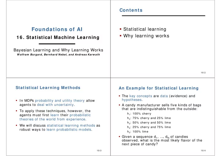

Contents � Statistical learning Foundations of AI � Why learning works 1 6 . Statistical Machine Learning Bayesian Learning and Why Learning Works W olfram Burgard, Bernhard Nebel, and Andreas Karw ath 10/ 1 10/ 2 Statistical Learning Methods An Exam ple for Statistical Learning � The key concepts are data (evidence) and hypotheses. � In MDPs probability and utility theory allow agents to deal with uncertainty. � A candy manufacturer sells five kinds of bags that are indistinguishable from the outside: � To apply these techniques, however, the h 1 : 100% cherry agents must first learn their probabilistic h 2 : 75% cherry and 25% lime theories of the world from experience. h 3 : 50% cherry and 50% lime � We will discuss statistical learning methods as h 4 : 25% cherry and 75% lime robust ways to learn probabilistic models. h 5 : 100% lime � Given a sequence d 1 , … , d N of candies observed, what is the most likely flavor of the next piece of candy? 10/ 3 10/ 4
Bayesian Learning Application of Bayes Rule � Let D represent all the data with observed value � Calculates the probability of each hypothesis, d . given the data. � The probability of each hypothesis is obtained by � It then makes predictions using all hypotheses Bayes rule: weighted by their probabilities (instead of a single best hypothesis). � The manufacturer tells us that the prior � Learning is reduced to probabilistic inference. distribution over h 1 , … , h 5 is given by < .1, .2, .4, .2, .1> � We compute the likelihood of the data under the assumption that the observations are independently and identically distributed (i.i.d.): 10/ 5 10/ 6 How to Make Predictions? Exam ple � Suppose we want to make predictions about � Suppose the bag is an all-lime bag ( h 5 ) � an unknown quantity X given the data d . The first 10 candies are all lime. Then P( d |h 3 ) is 0.5 10 because half the candies in an h 3 bag � are lime. � Evolution of the five hypotheses given 10 lime candies were observed (the values start at the prior!). � Predictions are weighted averages over the predictions of the individual hypotheses. � The key quantities are the hypothesis prior P(h i ) and the likelihood P(d|h i ) of the data under each hypothesis. 10/ 7 10/ 8
Maxim um a Posteriori ( MAP) Observations � A common approximation is to make predictions � The true hypothesis often dominates the based on a single most probable hypothesis. Bayesian prediction. � The maximum a posteriori (MAP) hypothesis is the � For any fixed prior that does not rule out the one that maximizes P(h i |d) . true hypothesis, the posterior of any false P ( X | d ) ≈ P ( X | h MAP ) hypothesis will eventually vanish. � In the candy example, h MAP = h 5 after three lime candies in a row. � The Bayesian prediction is optimal and, given � The MAP learner the predicts that the fourth candy the hypothesis prior, any other prediction will is lime with probability 1.0, whereas the Bayesian be correct less often. prediction is still 0.8. � It comes at a price that the hypothesis space � As more data arrive, MAP and Bayesian predictions can be very large or infinite. become closer. � Finding MAP hypotheses is often much easier than Bayesian learning. 10/ 9 10/ 10 W hy Learning W orks Maxim um -Likelihood Hypothesis ( ML) How can we decide that h is close to f when f is unknown? � A final simplification is to assume a uniform � Probably approximately correct prior over the hypothesis space. Stationarity as the basic assumption of PAC-Learning: � In that case MAP-learning reduces to choosing training and test sets are selected from the same the hypothesis that maximizes P(d|h i ) . population of examples with the same probability � This hypothesis is called the maximum- distribution. likelihood hypothesis (ML). Key question: how many examples do we need? � ML-learning is a good approximation to MAP X Set of examples learning and Bayesian learning when there is a D Distribution from which the examples are drawn Hypothesis space ( f ∈ uniform prior and when the data set is large. H H ) m Number of examples in the training set 10/ 11 10/ 12
Sam ple Com plexity PAC-Learning ⇒ Assumption: A hypothesis h is approximately correct if . P( h b is consistent with 1 example) To show: After the training period with m examples, with high probability, all consistent hypotheses are P( h b is consistent with N examples) approximately correct. P( H bad contains a consistent h ) Since | H bad | ≤ | H | P( H bad contains a consistent h ) We want to limit this probability by some small number δ : Since , we derive How high is the probability that a wrong hypothesis h b ∈ H bad Sample Complexity: Number of required examples, as a is consistent with the first m examples? function of and . 10/ 13 10/ 14 Sam ple Com plexity ( 2 ) Learning from Decision Lists In comparison to decision trees: Example: Boolean functions • The overall structure is simpler The number of Boolean functions over n attributes is • The individual tests are more complex | H | = 2 2 n . The sample complexity therefore grows as 2 n . Since the number of possible examples is also 2 n , any learning algorithm for the space of all Boolean This represents the hypothesis functions will do no better than a lookup table, if it merely returns a hypothesis that is consistent with all If we allow tests of arbitrary size, then any Boolean function can known examples. be represented. k-DL: Language with tests of length ≤ k . k-DT � k-DL 10/ 15 10/ 16
Sum m ary Learnability of k-DL ( Statistical Learning Methods) � Bayesian learning techniques formulate learning as a form of probabilistic inference. � Maximum a posteriori (MAP) learning selects the most likely hypothesis given the data. � Maximum likelihood learning selects the (Yes,No,no-Test,all permutations) hypothesis that maximizes the likelihood of the data. (Combination without repeating pos/ neg attributes) (with Euler’s summation formula) 10/ 17 10/ 18 Sum m ary ( Statistical Learning Theory) Inductive learning as learning the representation of a function from example input/ output pairs. � Decision trees learn deterministic Boolean functions. � PAC learning deals with the complexity of learning. � Decision lists as functions that are easy to learn. 10/ 19
Recommend
More recommend