Simple Linear Regression Regression models are used to study the - PowerPoint PPT Presentation
ST 370 Probability and Statistics for Engineers Simple Linear Regression Regression models are used to study the relationship of a response variable and one or more predictors . The response is also called the dependent variable , and the
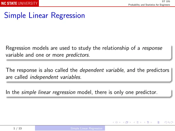
ST 370 Probability and Statistics for Engineers Simple Linear Regression Regression models are used to study the relationship of a response variable and one or more predictors . The response is also called the dependent variable , and the predictors are called independent variables . In the simple linear regression model, there is only one predictor. 1 / 13 Simple Linear Regression
ST 370 Probability and Statistics for Engineers Empirical Models Example: Oxygen and Hydrocarbon levels Production of oxygen Response: Y , purity of the produced oxygen (%); Predictor: x , level of hydrocarbons in part of the system (%). In R oxygen <- read.csv("Data/Table-11-01.csv") # scatter plot: plot(Purity ~ HC, oxygen) 2 / 13 Simple Linear Regression Empirical Models
ST 370 Probability and Statistics for Engineers The relationship between x and y is roughly linear, so we assume that Y = β 0 + β 1 x + ǫ for some coefficients β 0 (the intercept ) and β 1 (the slope ), where ǫ is a random noise term (or random error). The noise term ǫ is needed in the model, because without it the data points would have to fall exactly along a straight line, which they don’t. This is an empirical model, rather than a mechanistic model, because we have no physical or chemical mechanism to justify it. 3 / 13 Simple Linear Regression Empirical Models
ST 370 Probability and Statistics for Engineers What can we say about β 0 and β 1 ? By eye, the slope β 1 appears to be around (96 − 90) / (1 . 5 − 1 . 0) = 12, and β 0 appears to be around 90 − 1 . 0 × β 1 = 78. In R abline(a = 78, b = 12) This line over-predicts most of the data points with lower HC percentages, so perhaps it can be improved. 4 / 13 Simple Linear Regression Empirical Models
ST 370 Probability and Statistics for Engineers For any candidate values b 0 and b 1 , the predicted value for x = x i is b 0 + b 1 x i , and the observed value is y i , i = 1 , 2 , . . . , n . The residual is e i = observed − predicted = y i − ( b 0 + b 1 x i ) , i = 1 , 2 , . . . , n . The candidate values b 0 and b 1 are good if the residuals are generally small, and in particular if n n � � e 2 [ y i − ( b 0 + b 1 x i )] 2 L ( b 0 , b 1 ) = i = i =1 i =1 is small. 5 / 13 Simple Linear Regression Empirical Models
ST 370 Probability and Statistics for Engineers Least Squares Estimates The best candidates (in this sense) are the values of b 0 and b 1 that give the lowest value of L ( b 0 , b 1 ). They are the least squares estimates ˆ β 0 and ˆ β 1 and can be shown to be n � ( x i − ¯ x )( y i − ¯ y ) ˆ i =1 β 1 = n � x ) 2 ( x i − ¯ i =1 ˆ y − ˆ β 0 = ¯ β 1 ¯ x . 6 / 13 Simple Linear Regression Empirical Models
ST 370 Probability and Statistics for Engineers In R, the function lm() calculates least squares estimates: summary(lm(Purity ~ HC, oxygen)) The line labeled (Intercept) shows that ˆ β 0 = 74 . 283, and the line labeled HC shows that ˆ β 1 = 14 . 947. This line does indeed fit better than our initial candidate: abline(a = 74.283, b = 14.947, col = "red") # check the sums of squared residuals: L <- function(b0, b1) with(oxygen, sum((Purity - (b0 + b1 * HC))^2)) L(b0 = 78, b1 = 12) # 27.8985 L(b0 = 74.283, b1 = 14.947) # 21.24983 7 / 13 Simple Linear Regression Empirical Models
ST 370 Probability and Statistics for Engineers Estimating σ The regression equation also involves a third parameter σ , the standard deviation of the noise term ǫ . The least squares residuals are e i = y i − (ˆ β 0 + ˆ β 1 x i ) so the residual sum of squares is n � e 2 SS E = i . i =1 Because two parameters were estimated in finding the residuals, the residual degrees of freedom are n − 2, and the estimate of σ 2 is σ 2 = MS E = SS E ˆ n − 2 . 8 / 13 Simple Linear Regression Empirical Models
ST 370 Probability and Statistics for Engineers Other Estimates The sum of squared residuals is not the only criterion that could be used to measure the overall size of the residuals. One alternative is n n � � L 1 ( b 0 , b 1 ) = | e i | = | y i − ( b 0 + b 1 x i ) | . i =1 i =1 Estimates that minimize L 1 ( b 0 , b 1 ) have no closed form representation, but may be found by linear programming methods. They are used occasionally, but least squares estimates are generally preferred. 9 / 13 Simple Linear Regression Empirical Models
ST 370 Probability and Statistics for Engineers Sampling Variability The 20 observations in the oxygen data set are only one sample, and if other sets of 20 observations were made, the values would be at least a little different. The least squares estimates ˆ β 0 and ˆ β 1 would therefore also vary from sample to sample. We assume that there are true parameter values β 0 and β 1 and that if we carried out many experiments at a given level x , the responses Y would average out to β 0 + β 1 x . 10 / 13 Simple Linear Regression Empirical Models
ST 370 Probability and Statistics for Engineers The standard error measures how far an estimate might typically deviate from the true parameter value. Estimated standard errors may be calculated for ˆ β 0 and ˆ β 1 , and are shown in the R output. They are used to set up confidence intervals: ˆ β 1 ± t α/ 2 ,ν × estimated standard error is a 100(1 − α ) confidence interval for β 1 , where ν = n − 2 is the degrees of freedom for Residuals. 11 / 13 Simple Linear Regression Empirical Models
ST 370 Probability and Statistics for Engineers We can also test hypotheses: for example, there is no relationship between x and y if β 1 = 0. To test H 0 : β 1 = 0, we use ˆ β 1 t obs = estimated standard error and find the P -value as usual, as the probability of finding as large a value of | t obs | if H 0 were true. 12 / 13 Simple Linear Regression Empirical Models
ST 370 Probability and Statistics for Engineers The null hypothesis is not always β 1 = 0. For instance, previous operations might have suggested that β 1 = 12. To test H 0 : β 1 = 12, we use ˆ β 1 − 12 t obs = estimated standard error and in this case | t obs | = 2 . 238, and the probability that | T | ≥ 2 . 238 is 0.038. So we would reject this hypothesis at the α = 0 . 05 level, but not at the 0 . 01 level. 13 / 13 Simple Linear Regression Empirical Models
Recommend
More recommend
Explore More Topics
Stay informed with curated content and fresh updates.
