Simple Linear Regression Chapter 10 1 Motivation Have data - PDF document
4/29/2019 IMGD 2905 Simple Linear Regression Chapter 10 1 Motivation Have data (sample, x s) Want to know likely value B of next observation E.g., playtime versus skins owned A reasonable to compute mean (with Y
4/29/2019 IMGD 2905 Simple Linear Regression Chapter 10 1 Motivation • Have data (sample, x ’s) • Want to know likely value B of next observation – E.g., playtime versus skins owned • A – reasonable to compute mean (with Y confidence interval) A • B – could do same, but there appears to be relationship between X and Y! Predict B X e.g., “trendline” (regression) 2 1
4/29/2019 Motivation • Have data (sample, x ’s) • Want to know likely value of next observation B – E.g., playtime versus skins owned • A – reasonable to compute mean (with Y confidence interval) A • B – could do same, but there appears to be relationship between X and Y! Predict B X e.g., “trendline” (regression) 3 Motivation • Have data (sample, x ’s) • Want to know likely value B of next observation – E.g., playtime versus skins owned • A – reasonable to compute mean (with Y confidence interval) A • B – could do same, but there appears to be relationship between X and Y! Predict B X e.g., “trendline” (regression) 4 2
4/29/2019 Motivation • Have data (sample, x ’s) • Want to know likely value of next observation B – E.g., playtime versus skins owned • A – reasonable to compute mean (with Y confidence interval) A • B – could do same, but there appears to be relationship between X and Y! Predict B X e.g., “trendline” (regression) 5 Overview • Broadly, two types of prediction techniques: 1. Regression – mathematical equation to model, use model for predictions – We’ll discuss simple linear regression 2. Machine learning – branch of AI, use computer algorithms to determine relationships (predictions) – CS 453X Machine Learning 6 3
4/29/2019 Types of Regression Models • Explanatory variable explains dependent variable – Variable X (e.g., skill level) explains Y (e.g., KDA) – Can have 1 or 2+ • Linear if coefficients added, else Non-linear 7 Outline • Introduction (done) • Simple Linear Regression (next) – Linear relationship – Residual analysis – Fitting parameters • Measures of Variation • Misc 8 4
4/29/2019 Simple Linear Regression • Goal – find a linear relationship between to values – E.g., kills and skill, time and car speed • First, make sure relationship is linear! How? Scatterplot (c) no clear relationship (b) not a linear relationship (a) linear relationship – proceed with linear regression 9 Simple Linear Regression • Goal – find a linear relationship between to values – E.g., kills and skill, time and car speed • First, make sure relationship is linear! How? Scatterplot (c) no clear relationship (b) not a linear relationship (a) linear relationship – proceed with linear regression 10 5
4/29/2019 Linear Relationship • From algebra: line in form Y = mX + b – m is slope, b is y-intercept • Slope (m) is amount Y increases when X increases by 1 unit • Intercept (b) is where line crosses y-axis, or where y-value when x = 0 Y Y = mX + b Change m = Slope in Y Change in X b = Y-intercept X https://www.scribd.com/presentation/230686725/Fu-Ch11-Linear-Regression 11 Simple Linear Regression Example • Size of house related to its market value. X = square footage Y = market value ($) • Scatter plot (42 homes) indicates linear trend 12 6
4/29/2019 Simple Linear Regression Example • Two possible lines shown below (A and B) • Want to determine best regression line • Line A looks a better fit to data Y = mX + b – But how to know? 13 Simple Linear Regression Example • Two possible lines shown below (A and B) • Want to determine best regression line • Line A looks a better fit to data Y = mX + b – But how to know? Line that gives best fit to data is one that minimizes prediction error Least squares line (more later) 14 7
4/29/2019 Simple Linear Regression Example Chart • Scatterplot • Right click Add Trendline 15 Simple Linear Regression Example Formulas =SLOPE(C4:C45,B4:B45) • Slope = 35.036 =INTERCEPT(C4:C45,B4:B45) • Intercept = 32,673 • Estimate Y when X = 1800 square feet Y = 32,673 + 35.036 x (1800) = $95,737.80 16 8
4/29/2019 Simple Linear Regression Example • Market value = 32673 + 35.036 x (square feet) • Predicts market value better than just average But before use, examine residuals 17 Outline • Introduction (done) • Simple Linear Regression – Linear relationship (done) – Residual analysis (next) – Fitting parameters • Measures of Variation • Misc 18 9
4/29/2019 Residual Analysis • Before predicting, confirm that linear regression assumptions hold – Variation around line is normally distributed – Variation equal for all X – Variation independent for all X • How? Compute residuals (error in prediction) Chart 19 Residual Analysis https://www.qualtrics.com/support/stats-iq/analyses/regression-guides/interpreting-residual-plots-improve-regression/ 20 10
4/29/2019 Residual Analysis – Good https://www.qualtrics.com/support/stats-iq/analyses/regression-guides/interpreting-residual-plots-improve-regression/ Clustered towards middle Symmetrically distributed No clear pattern 21 Residual Analysis – Bad https://www.qualtrics.com/support/stats-iq/analyses/regression-guides/interpreting-residual-plots-improve-regression/ Clear shape Patterns Outliers Note: could do normality test (QQ plot) 22 11
4/29/2019 Residual Analysis – Summary • Regression assumptions: – Normality of variation around regression – Equal variation for all y values – Independence of variation ___________________ (a) ok (b) funnel (c) double bow (d) nonlinear 23 Outline • Introduction (done) • Simple Linear Regression – Linear relationship (done) – Residual analysis (done) – Fitting parameters (next) • Measures of Variation • Misc 24 12
4/29/2019 Linear Regression Model Y Y Y b m X i 0 i i i = r andom error Y b m X Observed value X X https://www.scribd.com/presentation/230686725/Fu-Ch11-Linear-Regression Random error associated with each observation 25 Fitting the Best Line • Plot all ( X i , Y i ) Pairs Y 60 40 20 0 X 0 20 40 60 https://www.scribd.com/presentation/230686725/Fu-Ch11-Linear-Regression 26 13
4/29/2019 Fitting the Best Line • Plot all ( X i , Y i ) Pairs • Draw a line. But how do we know it is best? Y 60 40 20 0 X 0 20 40 60 https://www.scribd.com/presentation/230686725/Fu-Ch11-Linear-Regression 27 Fitting the Best Line • Plot all ( X i , Y i ) Pairs • Draw a line. But how do we know it is best? Y Slope 60 changed 40 20 0 X Intercept 0 20 40 60 unchanged https://www.scribd.com/presentation/230686725/Fu-Ch11-Linear-Regression 28 14
4/29/2019 Fitting the Best Line • Plot all ( X i , Y i ) Pairs • Draw a line. But how do we know it is best? Slope Y unchanged 60 40 20 Intercept 0 X changed 0 20 40 60 https://www.scribd.com/presentation/230686725/Fu-Ch11-Linear-Regression 29 Fitting the Best Line • Plot all ( X i , Y i ) Pairs • Draw a line. But how do we know it is best? Slope Y changed 60 40 20 Intercept 0 X changed 0 20 40 60 https://www.scribd.com/presentation/230686725/Fu-Ch11-Linear-Regression 30 15
4/29/2019 Linear Regression Model • Relationship between variables is linear function Population Population Random Y-Intercept Slope Prediction Error Want error Y b m X as small as i 0 i i possible Dependent Independent (explanatory) (response) Variable Variable (e.g., skill level) (e.g., kills) 31 Least Squares Line • Want to minimize difference between actual y and predicted ŷ – Add up i for all observed y’s – But positive differences offset negative ones – (remember when this happened for variance?) Square the errors! Then, minimize (using Calculus) Minimize: Take derivative Set to 0 and solve https://cdn-images-1.medium.com/max/1600/1*AwC1WRm7jtldUcNMJTWmiA.png 32 16
4/29/2019 Least Squares Line Graphically n n 2 2 2 2 2 2 2 2 2 2 LS minimizes LS minimizes i i 1 1 2 2 3 3 4 4 i i 1 1 Y Y Y Y X X 2 2 0 0 1 1 2 2 2 2 ^ ^ 4 4 ^ ^ 2 2 ^ ^ 1 1 ^ ^ 3 3 Y Y X X i i 0 0 1 1 i i X X EPI 809/Spring 2008 33 https://www.scribd.com/presentation/230686725/Fu-Ch11-Linear-Regression 33 Least Squares Line Graphically https://www.desmos.com/calculator/zvrc4lg3cr 34 17
4/29/2019 Outline • Introduction (done) • Simple Linear Regression (done) • Measures of Variation (next) – Coefficient of Determination – Correlation • Misc 35 Measures of Variation • Several sources of variation in y Break this – Error in prediction (unexplained) down (next) – Variation from model (explained) 36 18
Recommend
More recommend
Explore More Topics
Stay informed with curated content and fresh updates.
