
SLIDE 1
1
Fitting a Model to Data
Reading: 15.1, 15.5.2
- Cluster image parts together by fitting a model to some
selected parts
- Examples:
– A line fits well to a set of points. This is unlikely to be due to chance, so we represent the points as a line. – A 3D model can be rotated and translated to closely fit a set of points or line segments. It it fits well, the object is recognized.
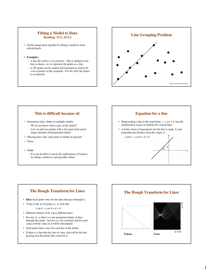
Line Grouping Problem
Slide credit: David Jacobs
This is difficult because of:
- Extraneous data: clutter or multiple models
– We do not know what is part of the model? – Can we pull out models with a few parts from much larger amounts of background clutter?
- Missing data: only some parts of model are present
- Noise
- Cost:
– It is not feasible to check all combinations of features by fitting a model to each possible subset
Equation for a line
- Representing a line in the usual form, y = mx + b, has the
problem that m goes to infinity for vertical lines
- A better choice of parameters for the line is angle, θ, and
perpendicular distance from the origin, d: x sin θ - y cos θ + d = 0
The Hough Transform for Lines
- Idea: Each point votes for the lines that pass through it.
- A line is the set of points (x, y) such that
x sin θ - y cos θ + d = 0
- Different choices of θ, d give different lines
- For any (x, y) there is a one parameter family of lines
through this point. Just let (x,y) be constants and for each value of θ the value of d will be determined.
- Each point enters votes for each line in the family
- If there is a line that has lots of votes, that will be the line