11. Regression and Least Squares Prof. Tesler Math 186 Winter 2019 - PowerPoint PPT Presentation
11. Regression and Least Squares Prof. Tesler Math 186 Winter 2019 Prof. Tesler Ch. 11: Linear Regression Math 186 / Winter 2019 1 / 24 Regression Given n points ( x 1 , y 1 ) , ( x 2 , y 2 ) , . . . , we want to determine a function y = f (
11. Regression and Least Squares Prof. Tesler Math 186 Winter 2019 Prof. Tesler Ch. 11: Linear Regression Math 186 / Winter 2019 1 / 24
Regression Given n points ( x 1 , y 1 ) , ( x 2 , y 2 ) , . . . , we want to determine a function y = f ( x ) that is close to them. Scatter plot of data (x,y) 50 ● 40 ● ● 30 ● ● y ● ● 20 ● 10 ● ● −20 −10 0 10 20 30 x Prof. Tesler Ch. 11: Linear Regression Math 186 / Winter 2019 2 / 24
Regression Based on knowledge of the underlying problem or on plotting the data, you have an idea of the general form of the function, such as: Polynomial y = β 0 + β 1 x + β 2 x 2 + β 3 x 3 Line y = β 0 + β 1 x 500 ! ! 100 ! ! ! ! ! ! ! 0 ! ! ! ! ! ! ! ! ! ! ! ! ! 80 ! ! − 1000 ! ! ! ! 60 10 12 14 16 18 20 5 10 15 20 25 Exponential Decay y = Ae − Bx Logistic Curve y = A / ( 1 + B / C x ) 10 ! ! ! ! ! ! ! ! ! ! ! ! 5 ! 8 ! 4 ! ! 6 3 ! ! ! 4 2 ! ! ! ! ! 1 2 ! ! ! ! ! ! ! ! ! ! ! ! ! ! ! ! ! ! ! ! ! ! ! ! 0 ! ! ! ! 0 0 5 10 15 20 25 30 0 5 10 15 20 Goal: Compute the parameters ( β 0 , β 1 , . . . or A , B , C , . . .) that give a “best fit” to the data. Prof. Tesler Ch. 11: Linear Regression Math 186 / Winter 2019 3 / 24
Regression The methods we consider require the parameters to occur linearly. It is fine if ( x , y ) do not occur linearly. y = β 0 + β 1 x + β 2 x 2 + β 3 x 3 E.g., plugging ( x , y ) = ( 2 , 3 ) into gives 3 = β 0 + 2 β 1 + 4 β 2 + 8 β 3 . For exponential decay, y = Ae − Bx , parameter B does not occur linearly. Transform the equation to: ln y = ln ( A ) − Bx = A ′ − Bx When we plug in ( x , y ) values, the parameters A ′ , B occur linearly. Transform the logistic curve y = A / ( 1 + B / C x ) to: � A � = ln ( B ) − x ln ( C ) = B ′ + C ′ x ln y − 1 x → ∞ y ( x ) . Now B ′ , C ′ occur linearly. where A is determined from A = lim Prof. Tesler Ch. 11: Linear Regression Math 186 / Winter 2019 4 / 24
Least squares fit to a line 50 ! 40 ! ! 30 ! ! y ! ! 20 ! 10 ! ! − 20 − 10 0 10 20 30 x Given n points ( x 1 , y 1 ) , ( x 2 , y 2 ) , . . . , we will fit them to a line ˆ y = β 0 + β 1 x : Independent variable: x . We assume the x ’s are known exactly or have negligible measurement errors. Dependent variable: y . We assume the y ’s depend on the x ’s but fluctuate due to a random process. We do not have y = f ( x ) , but instead, y = f ( x ) + error. Prof. Tesler Ch. 11: Linear Regression Math 186 / Winter 2019 5 / 24
Least squares fit to a line 50 ! 40 ! ! 30 ! ! y ! ! 20 ! 10 ! ! − 20 − 10 0 10 20 30 x Given n points ( x 1 , y 1 ) , ( x 2 , y 2 ) , . . . , we will fit them to a line ˆ y = β 0 + β 1 x : Predicted y value (on the line): y i = β 0 + β 1 x i ˆ Actual data ( • ): y i = β 0 + β 1 x i + ǫ i Residual (actual y minus prediction): ǫ i = y i − ˆ y i = y i − ( β 0 + β 1 x i ) Prof. Tesler Ch. 11: Linear Regression Math 186 / Winter 2019 6 / 24
Least squares fit to a line 50 ! 40 ! ! 30 ! ! y ! ! 20 ! 10 ! ! − 20 − 10 0 10 20 30 x We will use the least squares method : pick parameters β 0 , β 1 that minimize the sum of squares of the residuals. n � ( y i − ( β 0 + β 1 x i )) 2 L = i = 1 Prof. Tesler Ch. 11: Linear Regression Math 186 / Winter 2019 7 / 24
Least squares fit to a line n � ( y i − ( β 0 + β 1 x i )) 2 L = i = 1 � � ∂β 0 , ∂ L ∂ L To find β 0 , β 1 that minimize this, solve ∇ L = = ( 0 , 0 ) : ∂β 1 � � n n n � � � ∂ L = − 2 ( y i − ( β 0 + β 1 x i )) = 0 n β 0 + β 1 = ⇒ x i y i ∂β 0 i = 1 i = 1 i = 1 � � � � n n n n ∂ L � � � � 2 = − 2 ( y i − ( β 0 + β 1 x i )) x i = 0 β 0 + β 1 = ⇒ x i x i x i y i ∂β 1 i = 1 i = 1 i = 1 i = 1 which has solution (all sums are i = 1 to n ) β 1 = n ( � i x i y i ) − ( � i x i ) ( � � i y i ) i ( x i − ¯ x )( y i − ¯ y ) = β 0 = ¯ y − β 1 ¯ x � n ( � i x i 2 ) − ( � i x i ) 2 x ) 2 i ( x i − ¯ Not shown: use 2nd derivatives to confirm it’s a minimum rather than a maximum or saddle point. Prof. Tesler Ch. 11: Linear Regression Math 186 / Winter 2019 8 / 24
Best fitting line x = α 0 + α 1 y + ε y = β 0 + β 1 x + ε 50 50 y = 24.9494 + 0.6180x x = −28.2067 + 1.1501y slope = 0.6180 slope = 0.8695 ● ● 40 40 ● ● ● ● 30 30 ● ● ● ● y y ● ● ● ● 20 20 ● ● 10 10 ● ● ● ● −20 −10 0 10 20 30 −20 −10 0 10 20 30 x x The best fit for y = β 0 + β 1 x + error or x = α 0 + α 1 y + error give different lines! y = β 0 + β 1 x + error assumes the x ’s are known exactly with no errors, while the y ’s have errors. x = α 0 + α 1 y + error is the other way around. Prof. Tesler Ch. 11: Linear Regression Math 186 / Winter 2019 9 / 24
Total Least Squares / Principal Components Analysis x = # 0 + # 1 y + " y = ! 0 + ! 1 x + " 50 50 y = 24.9494 + 0.6180x x = − 28.2067 + 1.1501y slope = 0.6180 slope = 0.8695 ! ! 40 40 ! ! ! ! 30 30 ! ! ! ! y y ! ! ! ! 20 20 ! ! 10 10 ! ! ! ! − 20 − 10 0 10 20 30 − 20 − 10 0 10 20 30 x x First principal component All three of centered data 50 50 slope = 0.6934274 y = 25.99114 x = 1.685727 ! ! 40 40 ! ! ! ! 30 30 ! ! ! ! y y ! ! ! ! 20 20 ! ! 10 10 ! ! ! ! − 20 − 10 0 10 20 30 − 20 − 10 0 10 20 30 x x In many experiments, both x and y have measurement errors. Use Total Least Squares or Principal Components Analysis , in which the residuals are measured perpendicular to the line. Details require advanced linear algebra, beyond Math 18. Prof. Tesler Ch. 11: Linear Regression Math 186 / Winter 2019 10 / 24
Confidence intervals y = ! 0 + ! 1 x + " true line 150 sample data ! best fit line 95% prediction interval 100 ! ! ! ! y ! ! ! ! ! 50 r 2 = 0.7683551 0 5 10 15 20 25 x The best fit line — is different than the true line —. We found point estimates of β 0 and β 1 . Assuming errors are independent of x and normally distributed gives Confidence intervals for β 0 , β 1 . A prediction interval to extrapolate y = f ( x ) at other x ’s. Warning: it may diverge from the true line when we go out too far. Not shown: one can also do hypothesis tests on the values of β 0 and β 1 , and on whether two samples give the same line. Prof. Tesler Ch. 11: Linear Regression Math 186 / Winter 2019 11 / 24
Confidence intervals The method of least squares gave point estimates of β 0 and β 1 : β 1 = n � i x i y i − ( � i x i ) ( � � i y i ) i ( x i − ¯ x )( y i − ¯ y ) ˆ ˆ y − ˆ = β 0 = ¯ β 1 ¯ x � n ( � i x i 2 ) − ( � i x i ) 2 x ) 2 i ( x i − ¯ The sample variance of the residuals is n � 1 s 2 = ( y i − ( ˆ β 0 + ˆ β 1 x i )) 2 (with df = n − 2 ). n − 2 i = 1 100 ( 1 − α ) % confidence intervals: s √ � s √ � � � i x i 2 i x i 2 ˆ x ) , ˆ √ √ β 0 : β 0 − t α/ 2 , n − 2 β 0 + t α/ 2 , n − 2 n � n � i ( x i − ¯ i ( x i − ¯ x ) � � ˆ s x ) , ˆ s √ � √ � β 1 : β 1 − t α/ 2 , n − 2 β 1 + t α/ 2 , n − 2 i ( x i − ¯ i ( x i − ¯ x ) y at new x : ( ˆ y − w , ˆ y + w ) with ˆ y = β 0 + β 1 x � x ) 2 ( x − ¯ 1 + 1 and w = t α/ 2 , n − 2 · s · n + � x ) 2 i ( x i − ¯ Prof. Tesler Ch. 11: Linear Regression Math 186 / Winter 2019 12 / 24
Covariance Let X and Y be random variables, possibly dependent. Let µ X = E ( X ) , µ Y = E ( Y ) ��� �� 2 � Var ( X + Y ) = E (( X + Y − µ X − µ Y ) 2 ) = E � � X − µ X + Y − µ Y �� � 2 � �� � 2 � � � = E X − µ X + E Y − µ Y + 2 E ( X − µ X )( Y − µ Y ) = Var ( X ) + Var ( Y ) + 2 Cov ( X , Y ) where the covariance of X and Y is defined as � � Cov ( X , Y ) = E ( X − µ X )( Y − µ Y ) = E ( XY ) − E ( X ) E ( Y ) Independent variables have E ( XY ) = E ( X ) E ( Y ) , so Cov ( X , Y ) = 0 . But Cov ( X , Y ) = 0 does not guarantee X and Y are independent. Prof. Tesler Ch. 11: Linear Regression Math 186 / Winter 2019 13 / 24
Covariance and independence Independent variables have E ( XY ) = E ( X ) E ( Y ) , so Cov ( X , Y ) = 0 . But Cov ( X , Y ) = 0 does not guarantee X and Y are independent. Consider the standard normal distribution, Z . Z and Z 2 are dependent. Cov ( Z , Z 2 ) = E ( Z 3 ) − E ( Z ) E ( Z 2 ) . The standard normal distribution has mean 0: E ( Z ) = 0 . E ( Z 3 ) = 0 since Z 3 is an odd function and the pdf of Z is symmetric around Z = 0 . So Cov ( Z , Z 2 ) = 0 . Prof. Tesler Ch. 11: Linear Regression Math 186 / Winter 2019 14 / 24
Covariance properties We have Var ( X + Y ) = Var ( X ) + Var ( Y ) + 2 Cov ( X , Y ) where the covariance of X and Y is defined as � � Cov ( X , Y ) = E ( X − µ X )( Y − µ Y ) = E ( XY ) − E ( X ) E ( Y ) Additional properties of covariance Cov ( X , X ) = Var ( X ) Cov ( X , Y ) = Cov ( Y , X ) Cov ( aX + b , cY + d ) = ac Cov ( X , Y ) Prof. Tesler Ch. 11: Linear Regression Math 186 / Winter 2019 15 / 24
Recommend
More recommend
Explore More Topics
Stay informed with curated content and fresh updates.
