Data Combination in Particle Physics Correlated and non-Gaussian - PowerPoint PPT Presentation

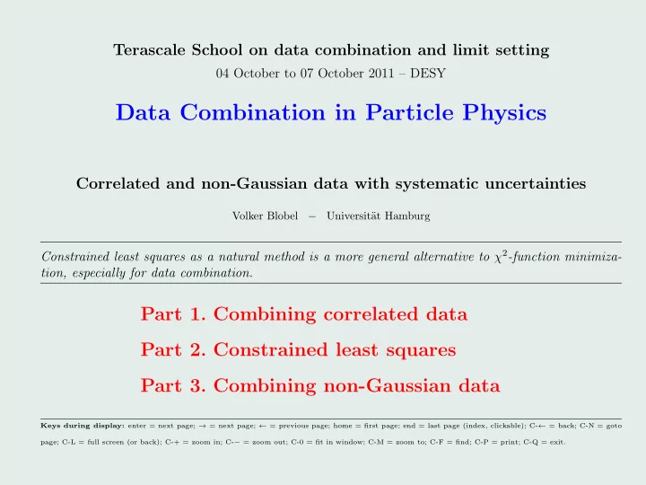
Terascale School on data combination and limit setting 04 October to 07 October 2011 – DESY Data Combination in Particle Physics Correlated and non-Gaussian data with systematic uncertainties Volker Blobel − Universit¨ at Hamburg Constrained least squares as a natural method is a more general alternative to χ 2 -function minimiza- tion, especially for data combination. Part 1. Combining correlated data Part 2. Constrained least squares Part 3. Combining non-Gaussian data Keys during display: enter = next page; → = next page; ← = previous page; home = first page; end = last page (index, clickable); C- ← = back; C-N = goto page; C-L = full screen (or back); C-+ = zoom in; C- − = zoom out; C-0 = fit in window; C-M = zoom to; C-F = find; C-P = print; C-Q = exit.

Part 1. Combining correlated data 1. Combining data 2. Averaging by linear least squares 3. Mean values, variances and covariances, correlations 4. Combining correlated data of a single quantity 5. Weights by Lagrange multiplier method 6. Least squares: Gauss, Legendre and Lagrange 7. Charm particle lifetime 8. Common additive systematic error I 9. Common multiplicative systematic error I 10. Average of two correlated data 11. Two-by-two covariance matrix from maximum likelihood 12. The two-dimensional normal distribution 13. Dzero result 14. Dzero: how big is the correlation coefficient? 15. Two alternative, but equivalent data combination methods 16. The PDG strategy V. Blobel – University of Hamburg Data Combination in Particle Physics page 2

1. Combining data For many physics analyses, several channels are combined into one result. In a similar way results from different experiments are merged. The aim of this procedure is to increase the precision of the results . . . no bias, as accurate as possible . . . Lifetime of charmed particles: four different values extracted with different methods from the same data – hence correlated Like-sign dimuon charge asymmetry: two values determined from different events samples – av- erage has significant deviation from the SM Mass of the top quark: several measured values with several systematic errors Non-linearity: e.g. normalization uncertainty: straightforward methods produce biased results Non-linearity: combining over-determined measurements of triangle parameters Non-Gaussian data: Poisson-distributed data, lognormal factors “Error” propagation: quantity depends on several measured values From linear problems with Gaussian variables . . . to non-linear problems with non-Gaussian variables and several sources of systematic errors. Essential: Understanding of physics, detector behaviour and data analysis. V. Blobel – University of Hamburg Data Combination in Particle Physics page 3

2. Averaging by linear least squares Weighted average: The average value x ave of single values x i , i = 1 , 2 , . . . n , with covariance matrix V x , is the weighted sum: � � x ave = w i x i with w i = 1 ( � x ave unbiased, if x i unbiased) i i where the weights w i are usually positive, but can be negative in certain cases. The weighted average according to the equation is unbiased, if the single values are unbiased: � � � E [ x ave ] = w i E [ x i ] = w i µ = µ for w i = 1 i i i The variance σ 2 ave follows from the law of (linear) propagation of uncertainties. Uncorrelated data x i ± σ i : ( V x diagonal) �� � − 1 �� � − 1 1 · 1 1 σ 2 w i = ave = σ 2 σ 2 σ 2 i i i i i V. Blobel – University of Hamburg Data Combination in Particle Physics page 4

3. Mean values, variances and covariances, correlations � 1-dim. random variable: mean value µ = E [ x ] = x · p ( x ) d x p ( x ) = pdf � � ( x − µ ) 2 � σ 2 = E ( x − µ ) 2 · p ( x ) d x . variance = V [ x ] = � � n -dim. random variable: mean value µ = E [ x ] = . . . x · p ( x ) d x � ( x − µ ) ( x − µ ) T � covariance matrix V x = E = V [ x ] . Random vector x , covariance matrix V x and correlation matrix C x :       x 1 σ 11 σ 12 . . . σ 1 n 1 ρ 12 . . . ρ 1 n       x 2 σ 21 σ 22 . . . σ 2 n ρ 21 1 . . . ρ 2 n             x = . . . V x = . . . . . . . . . C x = . . . . . . . . .             . . . . . . . . . . . . . . . . . . . . . x n σ n 1 σ n 2 . . . σ nn ρ n 1 ρ n 2 . . . 1 The elements ( V ) jk are the covariances ( V ) jk = σ jk = ρ jk σ j σ k , and ρ jk are the correlation coefficients with − 1 ≤ ρ jk ≤ +1 (values of the correlation coefficients are often printed in %). V. Blobel – University of Hamburg Data Combination in Particle Physics page 5

4. Combining correlated data of a single quantity needs inverse V − 1 Correlated data x i with (non-diagonal) covariance matrix V x : x �� � − 1 � n � � � � � ave = wV x w T = V − 1 V − 1 σ 2 w i = w i w j ( V x ) ij x x jk ij j,k j i,j =1 Optimal values of the weights are obtained by χ 2 -minimization (linear least squares). The inverse of V x is used as weight matrix in the weighted sum of squares: ( x = ( x 1 , x 2 , . . . x n ) T ) � � � S ( x ave ) = ( x ave · 1 − x ) T V − 1 V − 1 χ 2 -function x ( x ave · 1 − x ) = ( x ave − x i ) ij ( x ave − x j ) x i,j (all components of the vector 1 are one). The χ 2 -function S ( x ave ) is minimized with respect to the one parameter x ave . Generalization to different problems with multiple quantities possible, but constrained least squares is simpler. See NIMA A 500 (2003) 391–405); NIMA A 270 (1988) 110–117 V. Blobel – University of Hamburg Data Combination in Particle Physics page 6

. . . contnd. Correlated data x i with (non-diagonal) covariance matrix V x : The derivative of the weighted sum of squares S ( x ave ) with respect to the parameter x ave 1 ∂S = 1 T V − 1 x 1 · x ave − 1 T V − 1 x x 2 ∂x ave is set to zero to obtain the solution �� � � − 1 1 T V − 1 1 T V − 1 x ave = x 1 x = w x x The expression in []-parentheses is the weight w �� � − 1 � � � − 1 � � � � 1 T V − 1 1 T V − 1 V − 1 V − 1 w = x 1 w i = x x x jk ij � �� � � �� � j j,k row vector scalar The weight w is a 1-by- n matrix w = ( w 1 , w 2 . . . w n ) (or a row vector) and average value x ave and its variance σ 2 ave are given by n n � � ave = wV x w T = σ 2 x ave = w x = w i x i w i w j ( V x ) ij i =1 i,j =1 V. Blobel – University of Hamburg Data Combination in Particle Physics page 7

5. Weights by Lagrange multiplier method Alternative method for the determination of weights: Minimization of the variance σ 2 ave of the average n � ave = wV x w T = σ 2 w i w j ( V x ) ij i,j =1 subject to the equality constraint � w i = 1 i Method of Lagrange multipliers with Lagrange function: �� � � n L ( w , λ ) = w i w j ( V x ) ij + λ w i − 1 i,j =1 i with a single Lagrange multiplier λ . The constrained problem is solved by setting the derivative of L ( w , λ ) with respect to the weights w i and to the Lagrange multiplier λ to zero. The result is identical to the previous result. V. Blobel – University of Hamburg Data Combination in Particle Physics page 8

6. Least squares: Gauss, Legendre and Lagrange Carl Friedrich Gauß (1777 –1855) Used the least squares method already around 1794, but did not publish it at that time, but later in 1809. “Our principle, which we have made use of since 1795, has lately been published by Legendre . . . .” Proved in 1821 and 1823 the optimality of the least squares estimate without any assumptions that the random varibales follow a particular distribution (rediscovered by Markoff in 1912). Adrien-Marie Legendre (1752 – 1833) Was the first to publish the method in 1805. Joseph-Louis Lagrange (1736 –1813) Method of Lagrange multipliers (optimization of functions of several variables subject to equality constraints) formulated in “Le¸ cons sur le calcul des fonc- tions” (1804). Used the principle of minimizing the sum of the absolute residuals � i | r i | , with � i r i = 0 in 1799. Gauß-Markoff-Theorem: The vector x ∈ R n of measurements with a vector ǫ of random errors is assumed to be related to an unknown parameter (or parameters) by a fixed linear model relation. All el- ements ǫ i of ǫ have zero means (no bias), are uncorrelated and have the same variance. The residuals r i are the differences between the measured values x i and the values, given by the parametrization (linear model). The best (i.e. minimum variance) linear unbiased estimator (BLUE) for the parameter(s) is the least squares estimator, minimizing the sum of squared residuals || r || 2 . No assumptions are re- quired that the random errors follow a particular distribution; i.e. the normal (Gaussian) distribution is not required. V. Blobel – University of Hamburg Data Combination in Particle Physics page 9