BTRY 4090: Spring 2009 Theory of Statistics Guozhang Wang - PDF document

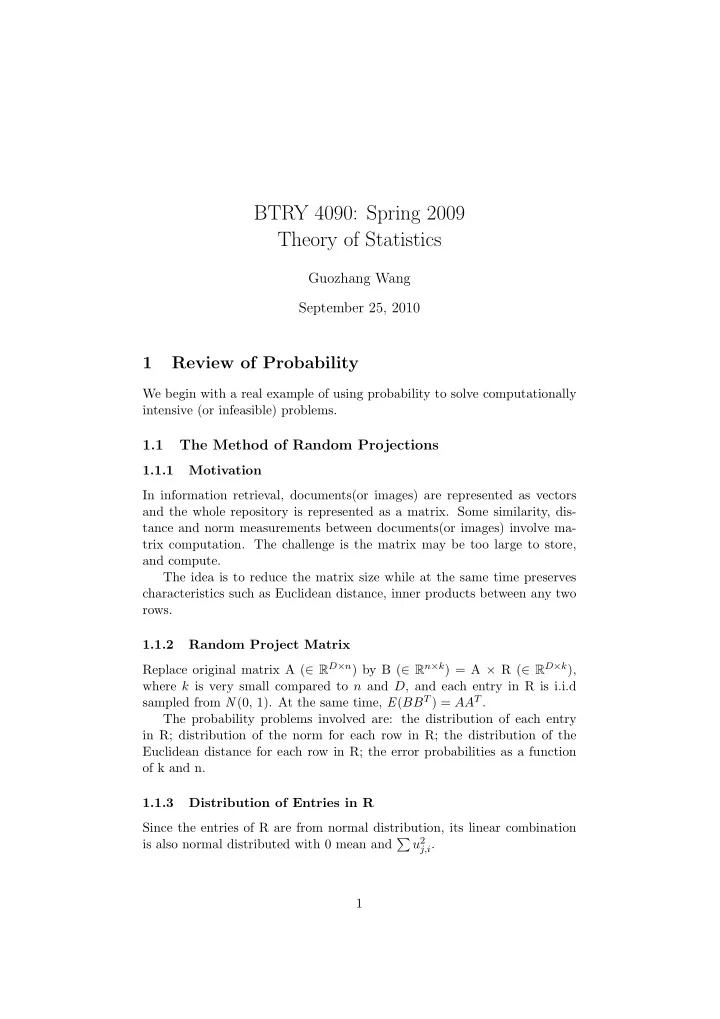
BTRY 4090: Spring 2009 Theory of Statistics Guozhang Wang September 25, 2010 1 Review of Probability We begin with a real example of using probability to solve computationally intensive (or infeasible) problems. 1.1 The Method of Random Projections 1.1.1 Motivation In information retrieval, documents(or images) are represented as vectors and the whole repository is represented as a matrix. Some similarity, dis- tance and norm measurements between documents(or images) involve ma- trix computation. The challenge is the matrix may be too large to store, and compute. The idea is to reduce the matrix size while at the same time preserves characteristics such as Euclidean distance, inner products between any two rows. 1.1.2 Random Project Matrix Replace original matrix A ( ∈ R D × n ) by B ( ∈ R n × k ) = A × R ( ∈ R D × k ), where k is very small compared to n and D , and each entry in R is i.i.d sampled from N (0, 1). At the same time, E ( BB T ) = AA T . The probability problems involved are: the distribution of each entry in R; distribution of the norm for each row in R; the distribution of the Euclidean distance for each row in R; the error probabilities as a function of k and n. 1.1.3 Distribution of Entries in R Since the entries of R are from normal distribution, its linear combination is also normal distributed with 0 mean and � u 2 j,i . 1

1.1.4 Distribution of Euclidean Norm From the computational formula, we know that V ar ( X ) = E ( X 2 ) − ( E ( X )) 2 , � k m 1 = 1 j =1 | v i,j | 2 . we can get an unbiased estimator of the Euclidean norm ˆ k Since v i,j is i.i.d., ˆ m 1 × k has a Chi-squared distribution with k degrees of freedom. And since we know that the mean for Chi-squared distribution is k , and m 1 = 2 × m 2 variance is 2 k , we can get the variance of ˆ 1 , where m 1 is the true k value. The coefficient of variation V ar ( ˆ m 1 ) = 2 k , which is independent of m 1 . m 2 1 This indicate that this is a good estimator with low relative variation. One note is that coefficient of variation has the assumption that the variation would increase as the real value itself increases. 1.1.5 Distribution of Euclidean Distance Has the similar result as the Euclidean Norm. 1.1.6 Estimation on Inner Product � k 1 The estimator of inner product j =1 v i,j v k,j is unbiased; however, the k variance is m 1 m 2 + a 2 , and thus the coefficient is not independent of a . One k simple illustration is that when two vectors are almost orthogonal (which is common in high dimension space, where two vectors are orthogonal with probability close to 1), a is close to 0, but coefficient of variation is close to infinity. Therefore random projections may not be good for estimating inner products. One note here is that this problem is due to the random sampling with entries of R, which is typical and hard to resolve. 1.1.7 Summary This elegant method is suitable for approximating Euclidean distances in massive, dense and heavy-tailed (some entries in certain rows are exces- sively large) data matrix; However, it does not take advantage of the data sparsity. Another note is that it has intrinsic relationship with SVM (which is aimed at solution sparsity, but not data sparsity; methods like PCA takes advantage of data sparsity). In real applications, the random matrix R can be applied only once. Since even we have multiple iterations of reduction and take the average value of estimators, the variance is the same. 2

1.2 Capture and Recapture Methods 1.2.1 Motivation Consider in the Database query cost estimating process, the order of the join operator is crucial to the query performance, and is dependent on the estimate on the size of intermediate results. The size of intermediate results can not be known exactly before the join is operated. However, by sampling the tuples and operate the ”mini-join” the sizes can be estimated using capturing and recapturing (sampling and mini join) methods. Note this method has several important assumptions: 1) the total pop- ulation does not change between capture and recapture; 2) the recapture process is random. 1.2.2 Estimation using Sampling The method has the following steps: 1. Use combination counting rules to compute the probability of the re- capture event. 2. After the probability is formalized as the function of the target popu- lation, compute maximum likelihood population. 3. The maximum likelihood value can be computed by observing the ratioofsuccessiveterms . Another way is plotting the curve and find the peak value (log form is suggested since the exponent arithmetic may be ”explosive”). 1.3 Bivariate Normal Distribution A good property of normal distribution is that if the joint distribution is normal, then the marginal and conditional distribution is also normal. Fur- thermore, the linear combination of normals is also normal. 1.3.1 Bivariate Normal to Random Projection Random projection utilizes this property to compute the variance of the unbiased estimators. Note here the variance of the estimator (which can also be treated as a random variable) is not the same as the variance of the population. The key idea is: E ( v 1 , v 2 ) 2 = E ( E ( v 2 1 , v 2 2 | v 2 )) = E ( v 2 2 × E ( v 2 1 | v 2 )) Note v 2 is treated as a constant when it is the dependent variable of the conditional distribution, and E ( v 2 1 | v 2 ) can be computed from E ( v 1 | v 2 ) and V ar ( v 1 | v 2 ). 3

1.3.2 Moment Generating Function (MGF) to Random Projec- tion MGF also can be utilized to simplify the computation of the estimators for random projection. The basic procedure has two steps: 1. Use some known MGF to derive the estimator’s MGF (for example, the function for normal distribution is exp ( µt + θ 2 t 2 / 2), for chi-square distribution is (1 − 2 t ) ( − k 2 )) 2. Use the MGF to get the n th moment of the estimator: M ( n ) = X E [ X n e tX ]. One note is that when the first moment (mean) of the estimator a is α , the n th moment of a − α is 0 only if the distribution is symmetric. 1.4 Tail Probabilities The tail probability P ( X > t ) or P ( | ¯ X − X | ≥ ǫX ) is extremely important, since it tells what is the probability that the error between the estimated value and the true value exceeds an ǫ fraction of the true value. Thus by studying how fast the error decreases, it can also imply the sample size to achieve some required accuracy. One note is that if the event is the same, then the probability is the same. On the other hand, it often requires numerical methods to exactly eval- uate P ( X > t ), and therefore one can give the tail probability upper bounds instead of the exact probability. 1.4.1 Tail Probability Inequalities Before we give several tail probability inequality theorems, we would like to note that each theorem have some assumptions which limit its applicability (eg, Markov’s Inequality assumes that the variable is non-negative and the first moment exists). Theorem 1.1 (Markov’s Inequality) If X is a random variable with P ( X ≥ 0) = 1 , and for which E(X) exists, then: P ( X ≥ t ) ≤ E ( X ) t Markov’s Inequality only uses the first moment and hence it is not very accurate. Theorem 1.2 (Chebyshev’s Inequality) Let X be random variable with mean µ and variance σ 2 . Then for any t > 0 : P ( | X − µ | ≥ t ) ≤ σ 2 t 2 4

Chebyshev’s Inequality only uses the second moment. One note is that making error depend on the variance may be more reasonable than making it depend on the mean (eg, if the mean is 0, then Markov’s Inequality is useless). Theorem 1.3 (Chernoff’s Inequality) Let X be a random variable with finite MGF M X ( t ) , then for any ǫ : P ( X ≥ ǫ ) ≤ e − tǫ M X ( t ) , for all t > 0 P ( X ≤ ǫ ) ≥ e − tǫ M X ( t ) , for all t < 0 The advantage of Chernoff’s Inequality is that by choosing different t , one can get a family of bounds on the distribution. Then by choosing t to minimize the upper bound, this usually leads to accurate probability bounds, which decrease exponentially fast . 1.4.2 Sample Size Selection Using Tail Bounds Since the variance of the estimator usually decrease with the number of samples (eg, the estimator of the mean of normal distribution is also nor- mally distributed with variance σ 2 k ). Thus by inputting this variance into the above inequality theorem, we can get the appropriate sample size to satisfy: P ( | ¯ X − µ | ≥ ǫµ ) ≤ δ for any δ . k is affected by • δ : level of significance, lower value causes larger k . σ 2 • µ 2 : noise/singal ratio, higher value causes larger k . • ǫ : accuracy, lower value causes larger k . 2 Limit Theorem 2.1 The Law of Large Numbers From the CLT, we can approximately get the rate of convergence of the X − µ ) 2 ) ≈ σ 2 LLN. Since ¯ X ≈ N ( µ, σ 2 /n ), we have V ar ( ¯ X ) = E (( ¯ n . Now we want to measure the error of the estimator by computing E ( | ¯ X − µ | ) (Note we do not use square here to have the same scale for estimator µ ). And from V ar ( ¯ σ X ) we get this expected value to be √ n . Therefore the rate 1 of the convergence of LLN is √ n . 5