Particle dynamics Particle overview Particle system Forces - PowerPoint PPT Presentation
Particle dynamics Particle overview Particle system Forces Constraints Second order motion analysis Particle system Particles are objects that have mass, position, and velocity, but without spatial extent
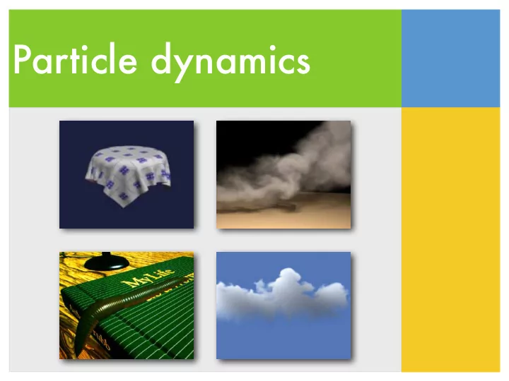
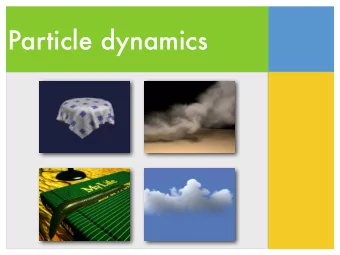
Particle dynamics
• Particle overview � • Particle system � • Forces � • Constraints � • Second order motion analysis
Particle system • Particles are objects that have mass, position, and velocity, but without spatial extent � • Particles are the easiest objects to simulate but they can be made to exhibit a wide range of objects
A Newtonian particle • First order motion is sufficient, if � • a particle state only contains position � • no inertia � • particles are extremely light � • Most likely particles have inertia and are affected by gravity and other forces � • This puts us in the realm of second order motion
Second-order ODE What is the differential equation that describes the behavior of a mass point? f = m a What does f depend on? x ( t ) = f ( x ( t ) , ˙ x ( t )) ¨ m
Second-order ODE x ( t ) = f ( x ( t ) , ˙ x ( t )) ¨ = f ( x , ˙ x ) m This is not a first oder ODE because it has second derivatives Add a new variable, v ( t ), to get a pair of coupled first order equations { ˙ x = v v = f /m ˙
Phase space ⎡ ⎤ x 1 x 2 Concatenate position and ⎢ ⎥ ⎢ ⎥ � � x x 3 ⎢ ⎥ velocity to form a 6-vector: = ⎢ ⎥ v v 1 ⎢ ⎥ position in phase space ⎢ ⎥ v 2 ⎣ ⎦ v 3 � ˙ � v � � First order differential equation: x = f ˙ velocity in the phase space v m
Quiz • A mass point attached to a spring obeys Hooke’s Law: f = -k (x - x0). What is the ODE that describes this motion?
• Particle overview � • Particle system � • Forces � • Constraints � • Second order motion analysis
Particle structure Particle x position a point in the phase space v velocity f force accumulator mass m
Solver interface solver � system interface solver 6 GetDim particle x x v Get/Set State v f v m Deriv Eval f m
Particle system structure system x 1 x 2 x n v n v 1 v 2 particles ... f n f 1 f 2 m n m 1 m 2 n time
Particle system structure solver � system solver interface 6n GetDim particles x 1 x 2 x n n time Get/Set State . . . v 1 v 2 v n v 1 v 2 v n Deriv Eval f 1 f 2 f n . . . m 1 m 2 m n
Deriv Eval Clear forces: loop over particles, zero force accumulator Calculate forces: sum all forces into accumulator Gather: loop over particles, copy v and f /m into destination array
• Particle overview � • Particle system � • Forces � • Constraints � • Second order motion analysis
Forces • Constant � • gravity � • Position dependent � • force fields, springs � • Velocity dependent � • drag
Particle systems with forces system x 1 x 2 x n v n v 1 v 2 particles ... f n f 1 f 2 m n m 1 m 2 � n time ... forces F 1 F 2 F m
Force structure • Unlike particles, forces are heterogeneous (type-dependent) � • Each force object “knows” � • which particles it influences � • how much contribution it adds to the force accumulator
Particle systems with forces system x 1 x 2 x n v n v 1 v 2 particles ... f n f 1 f 2 m n m 1 m 2 n time ... forces F 1 F 2 F m
Gravity x 1 x 2 x n Unary force: f = m G v 1 v 2 v n f 1 f 2 f n m 1 m 2 m n F Exerting a constant p force on each particle . . . sys apply_fun particle system G p->f += p->m*F->G
Viscous drag At very low speeds for small x 1 x 2 x n v 1 v 2 v n particles, air resistance is f 1 f 2 f n m 1 m 2 m n approximately: F p f drag = − k drag v . . . sys apply_fun particle system k p->f += p->v*F->k
Attraction Act on any or all pairs of particles, depending on their positions l f p = − k m p m q l x p | l | 2 | l | x q f q = − f p l = x p − x q
Attraction x p x q v p v q l f p = − k m p m q f p f q m p m q | l | 2 | l | F p sys apply_fun particle system k
Damped spring x p � � ˙ l · l l f p = − k s ( | l | − r ) + k d | l | | l | r f q = − f p | l | l = x p − x q x q
Damped spring x p x q v p v q � � ˙ l · l l f p f q f p = − k s ( | l | − r ) + k d | l | | l | m p m q F r p k d sys apply_fun particle system k s
Quiz For an ideal spring, what is the force it applies to two particles, p and q, attached to it. Write down the pseudo code for its “apply_fun”. x p x q v p v q f p f q m p m q F r p sys apply_fun particle system k s
Deriv Eval 1. Clear force accumulators x 1 x 2 x n v n v 1 v 2 2. Invoke apply_force ... f n f 1 f 2 functions m n m 1 m 2 ... F 1 F 2 F m 3. Return derivatives to solver � ˙ � v � � x = f ˙ v m
ODE solver Euler’s method: x ( t 0 + h ) = x ( t 0 ) + hf ( x , t ) x t +1 = x t + h ˙ x t v t +1 = v t + h ˙ v t
Euler step solver � system interface solver x t +1 = x t + h ˙ x t GetDim 3. particles v t +1 = v t + h ˙ v t 4. 2. x 1 x 2 x n 5. Advance time Get/Set State . . . v 1 v 2 v n time 1. v 1 v 2 v n Deriv Eval Deriv Eval f 1 f 2 f n . . . m 1 m 2 m n
• Particle overview � • Particle system � • Forces � • Constraints � • Second order motion analysis
Particle Interaction • We will revisit collision when we talk about rigid body simulation � • For now, just simple point-plane collisions
Collision detection Normal and tangential components x v T v N = ( N · v ) N N v N v T = v − v N v
Collision detection Particle is on the legal side if ( x − p ) · N ≥ 0 Particle is within of the wall if � x v T N ( x − p ) · N < � v N v Particle is heading in if p v · N < 0
Collision response Before After collision collision v ′ − k r v N v T v T v N v v ′ = v T − k r v N coefficient of restitution: 0 ≤ k r < 1
Contact Conditions for resting contact: 1. particle is on the collision surface 2. zero normal velocity If a particle is pushed into the contact plane a contact force f c is exerted to cancel the normal component of f N x v p f f N f T
• Particle overview � • Particle system � • Forces � • Constraints � • Second order motion analysis
Linear analysis • Linearly approximate acceleration � � � � d � x x x = f ( , t ) = A + a 0 v v v dt � � � � � d x 0 I x + a 0 = v − K − D v dt � • Split up analysis into different cases � • constant acceleration � • linear acceleration
Constant acceleration • Solution is � v ( t ) = v 0 + a 0 t � x ( t ) = x 0 + v 0 t + 1 2 a 0 t 2 � • v ( t ) only needs 1st order accuracy, but x ( t ) demands 2nd order accuracy
Linear acceleration • When K (or D) dominates ODE, what type of motion does it correspond to? � � � � � � � � � � d x 0 I x x = A = v − K − D v v dt � � • Need to compute the eigenvalues of A
Linear acceleration � � u 1 Assume is an eigenvalue of A , is the α u 2 corresponding eigenvector � � � � � � 0 I u 1 u 1 = α − K − D u 2 u 2 � � u The eigenvector of A has the form α u Assuming D is linear combination of K and I (Rayleigh damping) That means K and D have the same eigenvectors
Linear acceleration � � u For any u , if is an eigenvector of A, the following α u must be true � � � � � � 0 I u u = α − K − D α u α u Now assume u is an eigenvector for both K and D − λ k u − αλ d u = α 2 u � α = − 1 (1 2 λ d ) 2 − λ k 2 λ d ±
Eigenvalue approximation • If D dominates � α ≈ − λ d , 0 � • exponential decay � • If K dominates � √ � α ≈ ± λ k − 1 � • oscillation
Analysis • Constant acceleration (e.g. gravity) � • demands 2nd order accuracy for position � • Position dependence (e.g. spring force) � • demands stability, oscillatory motion � • looks at imaginary axis � • Velocity dependence (e.g. damping) � • demands stability, exponential decay � • looks at negative real axis
Explicit methods • First-order explicit Euler method � • constant acceleration: � bad (1st order) • position dependence: � very bad (unstable) • velocity dependence: � ok (conditionally stable) • RK3 and RK4 � • constant acceleration: � great (high order) • position dependence: � ok (conditionally stable) • velocity dependence: ok (conditionally stable)
Implicit methods • Implicit Euler method � • constant acceleration: � bad (1st order) • position dependence: � ok (stable but damped) • velocity dependence: � great (monotone) • Trapezoidal rule � • constant acceleration: � great (2nd order) • position dependence: � great (stable and no damp) • velocity dependence: good (stable, not monotone)
Recommend


More recommend
Explore More Topics
Stay informed with curated content and fresh updates.