1 Least Squares Regression Suppose someone hands you a stack of N - PDF document
Statistical Modeling and Analysis of Neural Data (NEU 560) Princeton University, Spring 2018 Jonathan Pillow Lecture 3B notes: Least Squares Regression 1 Least Squares Regression Suppose someone hands you a stack of N vectors, { x N } , each
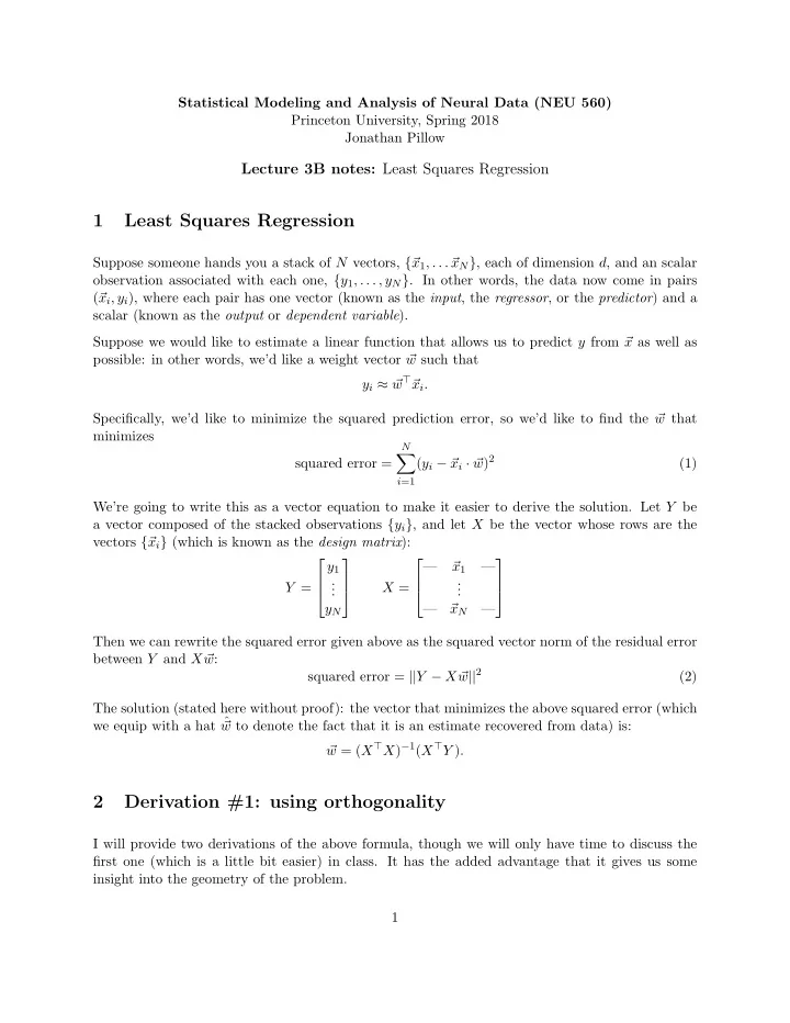
Statistical Modeling and Analysis of Neural Data (NEU 560) Princeton University, Spring 2018 Jonathan Pillow Lecture 3B notes: Least Squares Regression 1 Least Squares Regression Suppose someone hands you a stack of N vectors, { � x N } , each of dimension d , and an scalar x 1 , . . . � observation associated with each one, { y 1 , . . . , y N } . In other words, the data now come in pairs ( � x i , y i ), where each pair has one vector (known as the input , the regressor , or the predictor ) and a scalar (known as the output or dependent variable ). Suppose we would like to estimate a linear function that allows us to predict y from � x as well as possible: in other words, we’d like a weight vector � w such that w ⊤ � y i ≈ � x i . Specifically, we’d like to minimize the squared prediction error, so we’d like to find the � w that minimizes N � w ) 2 squared error = ( y i − � x i · � (1) i =1 We’re going to write this as a vector equation to make it easier to derive the solution. Let Y be a vector composed of the stacked observations { y i } , and let X be the vector whose rows are the vectors { � x i } (which is known as the design matrix ): — — y 1 x 1 � . . . . Y = X = . . y N — � x N — Then we can rewrite the squared error given above as the squared vector norm of the residual error between Y and X � w : w || 2 squared error = || Y − X � (2) The solution (stated here without proof): the vector that minimizes the above squared error (which we equip with a hat ˆ w to denote the fact that it is an estimate recovered from data) is: � w = ( X ⊤ X ) − 1 ( X ⊤ Y ) . � 2 Derivation #1: using orthogonality I will provide two derivations of the above formula, though we will only have time to discuss the first one (which is a little bit easier) in class. It has the added advantage that it gives us some insight into the geometry of the problem. 1
Let’s think about the design matrix X in terms of its d columns instead of its N rows. Let { X j } denote the j ′ th column, i.e., X = X 1 · · · X d (3) The columns of X span a d -dimensional subspace within the larger N -dimensional vector space that contains the vector Y . Generally Y does not lie exactly within this subspace. Least squares regression is therefore trying to find the linear combination of these vectors, X � w , that gets as close to possible to Y . What we know about the optimal linear combination is that it corresponds to dropping a line down from Y to the subspace spanned by { X 1 , . . . X D } at a right angle. In other words, the error vector ( Y − X � w ) (also known as the residual error ) should be orthogonal to every column of X : ( Y − X � w ) · X j = 0 , (4) for all columns j = 1 up to j = d . Written as a matrix equation this means: w ) ⊤ X = � ( Y − X � 0 (5) where � 0 is d -component vector of zeros. We should quickly be able to see that solving this for � w gives us the solution we were looking for: X ⊤ ( Y − X � w ) = X ⊤ Y − X ⊤ X � w = 0 (6) ( X ⊤ X ) � w = X ⊤ Y = ⇒ (7) w = ( X ⊤ X ) − 1 X ⊤ Y. = ⇒ (8) � So to summarize: the requirement that the residual errors Y − X � w be orthogonal to the columns of X was all we needed to derive the optimal weight vector � w . (Hooray!) 3 Derivation #2: Calculus 3.1 Calculus with Vectors and Matrices Here are two rules that will help us out for the second derivation of least-squares regression. First of all, let’s define what we mean by the gradient of a function f ( � x ) that takes a vector ( � x ) as its input. This is just a vector whose components are the derivatives with respect to each of the components of � x : ∂f ∂x 1 . ∇ f � . . ∂f ∂x d 2
Where ∇ (the “nabla” symbol) is what we use to denote gradient, though in practice I will often be lazy and write simply d f ∂ x or maybe x f . d� ∂� (Also, in case you didn’t know it, � is the symbol denoting “is defined as”). Ok, here are the two useful identities we’ll need: 1. Derivative of a linear function: ∂ ∂ ∂ a ⊤ � x ⊤ � x � a · � x = x � x = x � a = � a (9) ∂� ∂� ∂� d (If you think back to calculus, this is just like dx ax = a ). 2. Derivative of a quadratic function: if A is symmetric, then ∂ x ⊤ A� x � x = 2 A� x (10) ∂� dx ax 2 = 2 ax ). d (Again, thinking back to calculus this is just like If you ever need it, the more general rule (for non-symmetric A ) is: ∂ x ⊤ A� x = ( A + A ⊤ ) � x � x, ∂� which of course is the same thing as 2 A� x when A is symmetric. 3.2 Calculus Derivation We can call this derivation (i.e., the � w vector that minimizes the squared error defined above) the “straightforward calculus” derivation. We will differentiate the error with respect to � w , set it equal to zero (i.e., implying we have a local optimum of the error), and solve for � w . All we’re going to need is some algebra for pushing around terms in the error, and the vector calculus identities we put at the top. Let’s go! ∂ w SE = ∂ w ) ⊤ ( Y − X � w ( Y − X � w ) (11) ∂ � ∂ � = ∂ � � Y ⊤ Y − 2 � w ⊤ X ⊤ Y + � w ⊤ X ⊤ X � (12) w ∂ � w = − 2 X ⊤ Y + 2 X ⊤ X � w = 0 . (13) We can then solve this for � w as follows: X ⊤ X � w = X ⊤ Y (14) w = ( X ⊤ X ) − 1 X ⊤ Y = ⇒ (15) � 3
Easy, right? (Note: we’re assuming that X ⊤ X is full rank so that its inverse exists, implying that N > d and the rows are not all linearly dependent. ) 4
Recommend
More recommend
Explore More Topics
Stay informed with curated content and fresh updates.
