Linear least squares Non-consistent systems Ax = b , b / R ( A ) - PowerPoint PPT Presentation

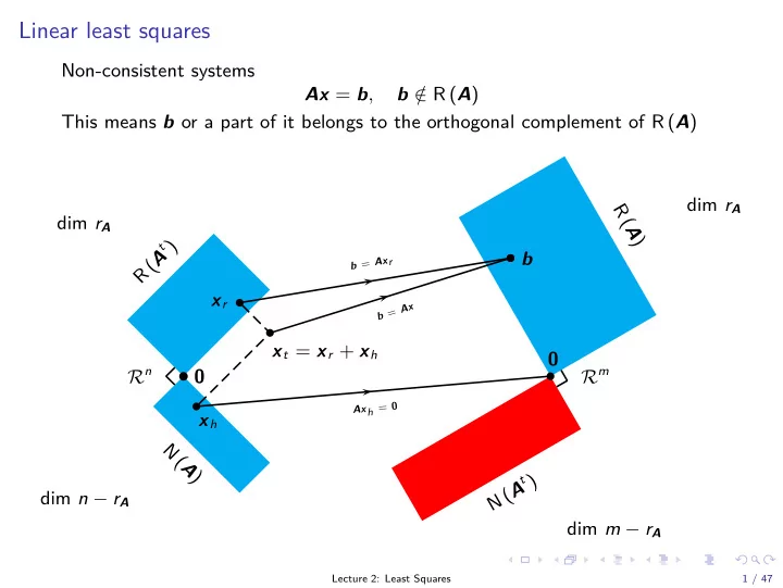
b Linear least squares Non-consistent systems Ax = b , b / ∈ R ( A ) This means b or a part of it belongs to the orthogonal complement of R ( A ) dim r A R ( A ) dim r A R ( A t ) b b = Ax r x r x A = b x t = x r + x h 0 R n R m b 0 Ax h = 0 x h N ( A ) N ( A t ) dim n − r A dim m − r A Lecture 2: Least Squares 1 / 47

Linear least squares Linear least squares for a deviation such that b + e ∈ R ( A ) Such a substitution creates a consistent system of equations (but e unknown!) Ax = b + e Vector of residuals e = Ax − b How to choose the vector of residuals in order to make the modified righthand side of the system of equations consistent? x ∈R q ( Ax − b ) t ( Ax − b ) min Lecture 2: Least Squares 2 / 47

Linear least squares optimization problem Least squares derivation n n n n � � � � x t A t Ax − 2 b t Ax + b t b = α ij β i ξ j + b t b γ ij ξ i ξ j − 2 i = 1 j = 1 i = 1 j = 1 where γ ij are the entries of A t A , β i the i th component of b and ξ i the i th component of x . Setting the derivative to zero w.r.t. ξ k amounts to solving n n � � γ ki ξ i − 2 2 α jk β j = 0 i = 1 j = 1 These n equations can be recast as ( A t A ) x = A t b These are called the normal equations. Lecture 2: Least Squares 3 / 47

Normal equations A t Ax = A t b ◮ Consistency rank � A t A � = rank � A t A A t b � ◮ Let x part be a particular solution, then so is x = x part + Xz ◮ What does x map to? A t e = A t ( Ax part − b ) = 0 so residuals are orthogonal to column space A or e ∈ N ( A t ) and Ax part is the orthogonal projection of b onto R ( A ) Lecture 2: Least Squares 4 / 47

Least squares solution We can split b as b = b 1 + b 2 , b 1 ∈ R ( A ) , b 2 ⊥ R ( A ) so we obtain e = ( Ax − b 1 ) − b 2 = − b 2 The minimal value for the objective function is e t e = ( Ax − b ) t ( Ax − b ) = b t ( I p − A ( A t A ) − 1 A t ) b Lecture 2: Least Squares 5 / 47

Least squares solution b a 1 p = Ax 0 a 2 R ( A ) Lecture 2: Least Squares 6 / 47

Computing the least squares solution matlab demo Avoid solving the normal equations! >> [A b] ans = 2.999999999980000 e+00 3.000000000010000 e+00 5.999999999990000 e+00 1.999999999990000 e+00 2.000000000000000 e+00 3.999999999990000 e+00 2.000000000020000 e+00 2.000000000010000 e+00 4.000000000030000 e+00 -9.999999999900000e-01 -1.000000000010000 e+00 -2.000000000000000 e+00 1.999999999970000 e+00 1.999999999960000 e+00 3.999999999930000 e+00 2.000000000000000 e+00 2.000000000000000 e+00 4.000000000000000 e+00 9.999999999800000 e-01 1.000000000030000 e+00 2.000000000010000 e+00 Whilst the linear system Ax = b is consistent mathematically ( b = a 1 + a 2 ), as evidenced by the singular values >> svd ([A b]) ans = 1.272792206132957 e+01 4.107364844986984 e-11 3.982911029842893 e-16 the square of the singular values in the matrix A t A produces a relative gap 1 , or larger than the machine precision ǫ m σ 2 2 ( A ) < σ 2 1 ( A ) ǫ m As a result, A t A cannot be inverted, and no solution is obtained. 1 This assumes we are working in double precision, where ǫ m ≈ 1 × 10 − 15 . Lecture 2: Least Squares 7 / 47

Least squares method and the SVD We involve the singular value decomposition of A � � � � � V t S 1 0 A = USV t = � 1 = U 1 S 1 V t U 1 U 2 V t 1 0 0 2 Applied to normal equations, this gives A t Ax = A t b gives ( V 1 S t SV t 1 ) x = V 1 SU t 1 b such that x = V 1 S − 1 U t 1 b + V 2 z ◮ Advantage over normal equations due to power of one of S (squareroot-free method), compared to S t S in the normal equations ◮ Operations reduced to orthogonal projection and scaling Lecture 2: Least Squares 8 / 47

Least squares method and the SVD matlab demo Finite precision acts as a nonlinearity, which may result in a different numerical rank for A than for A t A . Example: A = USV t where the singular values of A are σ 1 ( A ) = 1 , σ 2 ( A ) = 1 × 10 − 9 , σ 3 ( A ) = 0 and √ √ √ √ √     1 / 3 1 / 3 1 / 3 1 / 2 1 / 2 0 √ √ √ √ U = V = 1 / 2 − 1 / 2 0 − 1 / 2 0 1 / 2     √ √ √ 0 0 − 1 − 2 / 1 / 6 6 1 / 6 In matlab : >> A A = 4.082482908721113 e-01 -4.999999999999999e-01 2.886751340174626 e-01 4.082482900556147 e-01 -4.999999999999999e-01 2.886751351721632 e-01 0 0 0 Lecture 2: Least Squares 9 / 47

Least squares method and the SVD matlab demo The SVD of A is in agreement with the original decomposition, whereas the SVD of A t A truncates the dynamical range of the spectrum relative to σ 2 1 >> [U1 ,S1 ,V1] = svd(A); U1 , V1 , diag(S1)' U1 = -7.071067811865475e-01 -7.071067811865476e-01 0 -7.071067811865476e-01 7.071067811865475 e-01 0 0 0 1.000000000000000 e+00 V1 = -5.773502691896258e-01 -5.773502315590063e-01 -5.773503068202428e-01 7.071067811865475 e-01 4.608790676874364 e-08 -7.071067811865464e-01 -4.082482904638632e-01 8.164966075365897 e-01 -4.082482372461314e-01 ans = 9.999999999999999 e-01 9.999999462588933 e-10 0 >> [U2 ,S2 ,V2] = svd(A'*A); U2 , V2 , diag(S2)' U2 = -5.773502691896260e-01 -7.993060164940310e-01 1.666630092825368 e-01 7.071067811865475 e-01 -3.874131392520148e-01 5.915328051214906 e-01 -4.082482904638631e-01 4.593701683080254 e-01 7.888677847408841 e-01 V2 = -5.773502691896257e-01 7.242703261997147 e-01 3.769604239880175 e-01 7.071067811865475 e-01 6.743633567555686 e-01 -2.126830107586453e-01 -4.082482904638631e-01 1.437586785273193 e-01 -9.014803246224582e-01 ans = 1.000000000000000 e+00 5.019856335253205 e-17 1.772060549260711 e-17 Lecture 2: Least Squares 10 / 47

Least squares method and the SVD Assume unique least squares solution by rank ( A ) = q , then x = V 1 S − 1 U t 1 b r � v i 1 σ i u t = i b i = 1 = v 1 ( u t σ 1 ) + . . . + v r ( u t 1 r σ r ) Residuals follow by e = b − Ax = b − U 1 SV t 1 ( V 1 S − 1 U t 1 b ) = ( I − U 1 U t 1 ) b Lecture 2: Least Squares 11 / 47

Least squares method sensitivity Relative accuracy and sensitivity of the least squares solution Perturb b x + δ x = A † ( b + δ b ) Take δ b proportional relative to left singular vector u i , then � δ x � 2 � δ b � 2 = δ b t ( A † ) t A † δ b = 1 � δ b � 2 σ 2 i In the worst case, � δ b � is proportional to u q , the smallest singular value, if σ q � δ x � 2 = 1 � δ b � 2 σ 2 q Intuitive idea: we are working in the reverse direction, the inverse of the singular values of the mapping of domain of A to R ( A ) are the singular values of the inverse mapping from R ( A ) to R ( A t ) Lecture 2: Least Squares 12 / 47

Least squares method sensitivity Worst relative error magnification � δ x � 2 � x � 2 / � δ b � 2 � b � 2 δ b t ( A † ) t A † δ b max � b � 2 = max / � δ b � 2 b t ( A † ) t A † b b , δ b b , δ b = σ 2 1 σ 2 q Intuitive idea: a vector b with only a component in the direction of u 1 , resulting from the small x blown up by σ 1 , is perturbed by a vector δ b resulting from a large δ x made insignificant by σ n This number is called the condition number κ A = σ 1 ( A ) /σ n ( A ) Lecture 2: Least Squares 13 / 47

Least squares solution Exact solution x = ( A t A ) − 1 A t ˆ , a ∈ R ( A ) a � �� � ���� exact exact Noise distorts vector a into given data b = a + f x = ( A t A ) − 1 A t b = ( A t A ) − 1 A t a + ( A t A ) − 1 A t f Error on the solution x = ( A t A ) − 1 A t f x − ˆ Important to understand, vector e relates to the matrix A and its orthogonal complement, vector f however relates to the noise added to the exact vector a . Generally, f contains components in the R ( A ) , and thus f � = e Lecture 2: Least Squares 14 / 47

Least squares solution a + f 1 a + f 5 a + f 3 a + f 4 a a + f 6 a + f 2 R ( A ) Lecture 2: Least Squares 15 / 47

Least squares solution b = a + f 1 ˆ b = a − e A ˆ x = b + e Ax = a R ( A ) Lecture 2: Least Squares 16 / 47

Least squares statistical properties First order and second order assumptions x ] = ( A t A ) − 1 E [ f ] = 0 E [ x − ˆ (1) E � x ) t � = ( A t A ) − 1 σ 2 ( x − ˆ x )( x − ˆ (2) ◮ unbiasedness : repeating a large number of experiments using the same exact data a and A but different noise realizations of f (white noise), their average will be equal to the exact solution a ◮ error covariance : while the estimate is unbiased, certain directions in R n are estimated more accurately than others (see sensitivity) Lecture 2: Least Squares 17 / 47

White noise Example: A ∈ R 100 × 2 , a ∈ R 100 , find least squares solution to Ax = a + f with f ∈ R 100 and E [ f f t ] = ( 0 . 1 ) 2 I If δ x = x − ˆ x , we find E � δ x δ x t � = VS − 2 V t σ 2 (3) E � � SV t δ x � � = σ (4) Lecture 2: Least Squares 18 / 47

White noise matlab demo Case 1: � � � � 1 . 2247 0 0 . 6731 − 0 . 7396 S = , V = 0 1 − 0 . 7396 − 0 . 6731 Take x exact = v 1 + v 2 and compute eigenvalues of E � ( x − x exact )( x − x exact ) t � for 500 samples of b : � � 0 . 0087 0 . 0021 Λ = { 0 . 0062 , 0 . 0105 } 0 . 0021 0 . 0079 giving a relative accuracy of 1 . 2987 ≈ 1 . 2247 Lecture 2: Least Squares 19 / 47