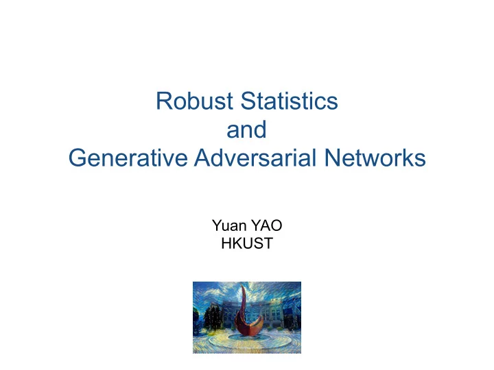
Robust Statistics and Generative Adversarial Networks Yuan YAO - PowerPoint PPT Presentation

Multi-task Regression Depth � Y | X ∼ N ( B T X, � 2 I m ) ( X, Y ) ∼ P B : X ∼ N (0 , Σ ) , ( X 1 , Y 1 ) , ..., ( X n , Y n ) ∼ (1 − ✏ ) P B + ✏ Q Theorem [G17]. For some C > 0 , B � B ))  C � 2 ⇣ pm n _ ✏ 2 ⌘ B � B ) T Σ ( b Tr (( b , ⇣ pm n _ ✏ 2 ⌘ F  C � 2 k b B � B k 2 ,  2 � � �� with high probability uniformly over . B, Q

Covariance Matrix X 1 , ..., X n ⇠ (1 � ✏ ) N (0 , Σ ) + ✏ Q . How to estimate Σ ?

Covariance Matrix X 1 , ..., X n ⇠ (1 � ✏ ) N (0 , Σ ) + ✏ Q . How to estimate Σ ? how to estimate ?

Covariance Matrix

Covariance Matrix

Covariance Matrix

Covariance Matrix

Covariance Matrix

Covariance Matrix ( n n ) 1 I {| u T X i | 2 � u T Γ u } , 1 I {| u T X i | 2 < u T Γ u } X X D ( Γ , { X i } n i =1 ) = min k u k =1 min n n i =1 i =1

Covariance Matrix ( n n ) 1 I {| u T X i | 2 � u T Γ u } , 1 I {| u T X i | 2 < u T Γ u } X X D ( Γ , { X i } n i =1 ) = min k u k =1 min n n i =1 i =1 ˆ Γ ⌫ 0 D ( Γ , { X i } n Σ = ˆ ˆ Γ = arg max i =1 ) Γ / � ,

Covariance Matrix ( n n ) 1 I {| u T X i | 2 � u T Γ u } , 1 I {| u T X i | 2 < u T Γ u } X X D ( Γ , { X i } n i =1 ) = min k u k =1 min n n i =1 i =1 ˆ Γ ⌫ 0 D ( Γ , { X i } n Σ = ˆ ˆ Γ = arg max i =1 ) Γ / � , Theorem [CGR15]. For some C > 0 , ⇣ p n _ ✏ 2 ⌘ k ˆ Σ � Σ k 2 op  C with high probability uniformly over . Σ , Q

Summary ⇣ p n _ ✏ 2 ⌘ k · k 2 mean � 2 _ � 2 reduced rank r ( p + m ) k · k 2  2 ✏ 2 regression F  2 n s 2 log( ep/s ) Gaussian graphical k · k 2 _ s ✏ 2 ` 1 model n ⇣ p n _ ✏ 2 ⌘ k · k 2 covariance matrix op _ ✏ 2 s log( ep/s ) k · k 2 sparse PCA F n � 2 � 2

Summary ⇣ p n _ ✏ 2 ⌘ k · k 2 mean � 2 _ � 2 reduced rank r ( p + m ) k · k 2  2 ✏ 2 regression F  2 n s 2 log( ep/s ) Gaussian graphical k · k 2 _ s ✏ 2 ` 1 model n ⇣ p n _ ✏ 2 ⌘ k · k 2 covariance matrix op _ ✏ 2 s log( ep/s ) k · k 2 sparse PCA F n � 2 � 2

Computation

Computational Challenges X 1 , ..., X n ⇠ (1 � ✏ ) N ( ✓ , I p ) + ✏ Q . How to estimate ✓ ?

Computational Challenges X 1 , ..., X n ⇠ (1 � ✏ ) N ( ✓ , I p ) + ✏ Q . How to estimate ✓ ? Lai, Rao, Vempala Diakonikolas, Kamath, Kane, Li, Moitra, Stewart Balakrishnan, Du, Singh Dalalyan, Carpentier, Collier, Verzelen

Computational Challenges X 1 , ..., X n ⇠ (1 � ✏ ) N ( ✓ , I p ) + ✏ Q . How to estimate ✓ ? Lai, Rao, Vempala Diakonikolas, Kamath, Kane, Li, Moitra, Stewart Balakrishnan, Du, Singh Dalalyan, Carpentier, Collier, Verzelen • Polynomial algorithms are proposed [Diakonikolas et al.’16, Lai et al. 16] of minimax optimal statistical precision • needs information on second or higher order of moments • some priori knowledge about ✏

Advantages of Tukey Median • A well-defined objective function ✏ • Adaptive to and Σ • Optimal for any elliptical distribution

Advantages of Tukey Median • A well-defined objective function ✏ • Adaptive to and Σ • Optimal for any elliptical distribution

Advantages of Tukey Median • A well-defined objective function ✏ • Adaptive to and Σ • Optimal for any elliptical distribution

Advantages of Tukey Median • A well-defined objective function ✏ • Adaptive to and Σ • Optimal for any elliptical distribution

A practically good algorithm?

Generative Adversarial Networks [Goodfellow et al. 2014] men- we , lin- al- exceeds the Note: R-package for Tukey median can not deal with more than 10 dimensions [https://github.com/ChenMengjie/ DepthDescent]

Robust Learning of Cauchy Distributions Table 4: Comparison of various methods of robust location estimation under Cauchy distributions. Samples are drawn from (1 � ✏ ) Cauchy (0 p , I p ) + ✏ Q with ✏ = 0 . 2 , p = 50 and various choices of Q . Sample size: 50,000. Discriminator net structure: 50-50-25-1. Generator g ω ( ⇠ ) structure: 48-48-32-24-12-1 with absolute value activation function in the output layer. Contamination Q JS-GAN ( G 1 ) JS-GAN ( G 2 ) Dimension Halving Iterative Filtering Cauchy (1 . 5 ⇤ 1 p , I p ) 0.0664 (0.0065) 0.0743 (0.0103) 0.3529 (0.0543) 0.1244 (0.0114) Cauchy (5 . 0 ⇤ 1 p , I p ) 0.0480 (0.0058) 0.0540 (0.0064) 0.4855 (0.0616) 0.1687 (0.0310) Cauchy (1 . 5 ⇤ 1 p , 5 ⇤ I p ) 0.0754 (0.0135) 0.0742 (0.0111) 0.3726 (0.0530) 0.1220 (0.0112) Normal (1 . 5 ⇤ 1 p , 5 ⇤ I p ) 0.0702 (0.0064) 0.0713 (0.0088) 0.3915 (0.0232) 0.1048 (0.0288)) • Dimension Halving: [Lai et al.’16] https://github.com/kal2000/AgnosticMeanAndCovarianceCode . • Iterative Filtering: [Diakonikolas et al.’17] https://github.com/hoonose/robust-filter .

f-GAN Given a strictly convex function f that satisfies f (1) = 0, the f -divergence between two probability distributions P and Q is defined by ✓ p ◆ Z D f ( P k Q ) = dQ . (8) f q Let f ⇤ be the convex conjugate of f . A variational lower bound of (8) is [ E P T ( X ) � E Q f ⇤ ( T ( X ))] . D f ( P k Q ) � sup (9) T 2 T where equality holds whenever the class T contains the function f 0 ( p / q ). [Nowozin-Cseke-Tomioka’16] f -GAN minimizes the variational lower bound (9) " # n X 1 b T ( X i ) � E Q f ⇤ ( T ( X )) P = arg min sup . (10) n Q 2 Q T 2 T i =1 with i.i.d. observations X 1 , ..., X n ⇠ P .

From f-GAN to Tukey’s Median: f-learning Consider the special case ⇢ ✓ e ◆ � q q 2 e f 0 T = : e Q (11) . q which is tight if P 2 e Q . The sample version leads to the following f -learning " ◆◆# ✓ e ◆ ✓ ✓ e n X 1 q ( X i ) q ( X ) b f 0 � E Q f ⇤ f 0 P = arg min sup (12) q ( X i ) q ( X ) . n Q 2 Q Q 2 e e Q i =1 • If f ( x ) = x log x , Q = e Q , (12) ) Maximum Likelihood Estimate R • If f ( x ) = ( x � 1)+, then D f ( P k Q ) = 1 | p � q | is the TV-distance, 2 f ⇤ ( t ) = t I { 0  t  1 } , f -GAN ) TV-GAN r ! 0 • Q = { N ( η , I p ) : η 2 R p } and e Q = { N ( e η , I p ) : k e η � η k  r } , (12) ) Tukey’s Median

f-Learning

f-Learning ✓ p ◆ Z f-divergence D f ( P k Q ) = f dQ. q

f-Learning ✓ p ◆ Z f-divergence D f ( P k Q ) = f dQ. q ( tu � f ⇤ ( t )) , f ( u ) = sup t

f-Learning ✓ p ◆ Z f-divergence D f ( P k Q ) = f dQ. q variational [ E X ⇠ P T ( X ) � E X ⇠ Q f ⇤ ( T ( X ))] ) = sup representation T

f-Learning ✓ p ◆ Z f-divergence D f ( P k Q ) = f dQ. q variational [ E X ⇠ P T ( X ) � E X ⇠ Q f ⇤ ( T ( X ))] ) = sup representation T ✓ p ( x ) ◆ T ( x ) = f 0 optimal T q ( x )

f-Learning ✓ p ◆ Z f-divergence D f ( P k Q ) = f dQ. q variational [ E X ⇠ P T ( X ) � E X ⇠ Q f ⇤ ( T ( X ))] ) = sup representation T ( ! !!) d ˜ d ˜ Q ( X ) Q ( X ) E X ⇠ P f 0 � E X ⇠ Q f ⇤ f 0 = sup dQ ( X ) dQ ( X ) ˜ Q

f-Learning ( ) Z n X 1 f ⇤ ( T ) dQ f-GAN Q 2 Q max min T ( X i ) � n T 2 T i =1 ( ) ✓ ˜ ◆ ✓ ✓ ˜ ◆◆ Z n X 1 q ( X i ) q f 0 f ⇤ f 0 Q 2 Q max min � dQ , f-Learning q ( X i ) n q Q 2 ˜ ˜ Q i =1

f-Learning ( ) Z n X 1 f ⇤ ( T ) dQ f-GAN Q 2 Q max min T ( X i ) � n T 2 T i =1 ( ) ✓ ˜ ◆ ✓ ✓ ˜ ◆◆ Z n X 1 q ( X i ) q f 0 f ⇤ f 0 Q 2 Q max min � dQ , f-Learning q ( X i ) n q Q 2 ˜ ˜ Q i =1

f-Learning ( ) Z n X 1 f ⇤ ( T ) dQ f-GAN Q 2 Q max min T ( X i ) � n T 2 T i =1 ( ) ✓ ˜ ◆ ✓ ✓ ˜ ◆◆ Z n X 1 q ( X i ) q f 0 f ⇤ f 0 Q 2 Q max min � dQ , f-Learning q ( X i ) n q Q 2 ˜ ˜ Q i =1

f-Learning ( ) Z n X 1 f ⇤ ( T ) dQ f-GAN Q 2 Q max min T ( X i ) � n T 2 T i =1 ( ) ✓ ˜ ◆ ✓ ✓ ˜ ◆◆ Z n X 1 q ( X i ) q f 0 f ⇤ f 0 Q 2 Q max min � dQ , f-Learning q ( X i ) n q Q 2 ˜ ˜ Q i =1 [Nowozin, Cseke, Tomioka]

f-Learning Jensen-Shannon GAN f ( x ) = x log x � ( x + 1) log( x + 1) . Kullback-Leibler f ( x ) = x log x MLE f ( x ) = 2 � 2 p x , Hellinger Squared rho Total Variation depth f ( x ) = ( x � 1) + [Goodfellow et al., Baraud and Birge]

f-Learning Jensen-Shannon GAN f ( x ) = x log x � ( x + 1) log( x + 1) . Kullback-Leibler f ( x ) = x log x MLE f ( x ) = 2 � 2 p x , Hellinger Squared rho Total Variation depth f ( x ) = ( x � 1) + [Goodfellow et al., Baraud and Birge]

f-Learning Jensen-Shannon GAN f ( x ) = x log x � ( x + 1) log( x + 1) . Kullback-Leibler f ( x ) = x log x MLE f ( x ) = 2 � 2 p x , Hellinger Squared rho Total Variation depth f ( x ) = ( x � 1) + [Goodfellow et al., Baraud and Birge]

f-Learning Jensen-Shannon GAN f ( x ) = x log x � ( x + 1) log( x + 1) . Kullback-Leibler f ( x ) = x log x MLE f ( x ) = 2 � 2 p x , Hellinger Squared rho Total Variation depth f ( x ) = ( x � 1) + [Goodfellow et al., Baraud and Birge]

f-Learning Jensen-Shannon GAN f ( x ) = x log x � ( x + 1) log( x + 1) . Kullback-Leibler f ( x ) = x log x MLE f ( x ) = 2 � 2 p x , Hellinger Squared rho Total Variation depth f ( x ) = ( x � 1) + [Goodfellow et al., Baraud and Birge]

TV-Learning ( ◆) ⇢ ˜ � ✓ ˜ n X 1 q ( X i ) q Q 2 Q max min q ( X i ) � 1 q � 1 � Q I n Q 2 ˜ ˜ Q i =1

TV-Learning ( ◆) ⇢ ˜ � ✓ ˜ n X 1 q ( X i ) q Q 2 Q max min q ( X i ) � 1 q � 1 � Q I n Q 2 ˜ ˜ Q i =1 n o n N ( ✓ , I p ) : ✓ 2 R p o ˜ N (˜ ✓ , I p ) : ˜ Q = ✓ 2 N r ( ✓ ) Q =

TV-Learning ( ◆) ⇢ ˜ � ✓ ˜ n X 1 q ( X i ) q Q 2 Q max min q ( X i ) � 1 q � 1 � Q I n Q 2 ˜ ˜ Q i =1 n o n N ( ✓ , I p ) : ✓ 2 R p o ˜ N (˜ ✓ , I p ) : ˜ Q = ✓ 2 N r ( ✓ ) Q = r ! 0

TV-Learning ( ◆) ⇢ ˜ � ✓ ˜ n X 1 q ( X i ) q Q 2 Q max min q ( X i ) � 1 q � 1 � Q I n Q 2 ˜ ˜ Q i =1 n o n N ( ✓ , I p ) : ✓ 2 R p o ˜ N (˜ ✓ , I p ) : ˜ Q = ✓ 2 N r ( ✓ ) Q = r ! 0 n 1 u T X i � u T θ X � max θ 2 R min I Tukey depth n k u k =1 i =1

TV-Learning ( ◆) ⇢ ˜ � ✓ ˜ n X 1 q ( X i ) q Q 2 Q max min q ( X i ) � 1 q � 1 � Q I n Q 2 ˜ ˜ Q i =1

TV-Learning ( ◆) ⇢ ˜ � ✓ ˜ n X 1 q ( X i ) q Q 2 Q max min q ( X i ) � 1 q � 1 � Q I n Q 2 ˜ ˜ Q i =1 n N (0 , Σ ) : Σ 2 R p ⇥ p o n o Σ = Σ + ruu T , k u k = 1 ˜ N (0 , ˜ Σ ) : ˜ Q = Q =

TV-Learning ( ◆) ⇢ ˜ � ✓ ˜ n X 1 q ( X i ) q Q 2 Q max min q ( X i ) � 1 q � 1 � Q I n Q 2 ˜ ˜ Q i =1 n N (0 , Σ ) : Σ 2 R p ⇥ p o n o Σ = Σ + ruu T , k u k = 1 ˜ N (0 , ˜ Σ ) : ˜ Q = Q = r ! 0

TV-Learning ( ◆) ⇢ ˜ � ✓ ˜ n X 1 q ( X i ) q Q 2 Q max min q ( X i ) � 1 q � 1 � Q I n Q 2 ˜ ˜ Q i =1 n N (0 , Σ ) : Σ 2 R p ⇥ p o n o Σ = Σ + ruu T , k u k = 1 ˜ N (0 , ˜ Σ ) : ˜ Q = Q = r ! 0 (related to) matrix depth " ! !# n n X X 1 1 I {| u T X i | 2  u T Σ u } � P ( � 2 I {| u T X i | 2 > u T Σ u } � P ( � 2 max min 1  1) ^ 1 > 1) n n Σ k u k =1 i =1 i =1

robust deep statistics learning community community

robust deep f-Learning statistics learning f-GAN community community

robust deep f-Learning statistics learning f-GAN community community practically good algorithms

theoretical foundation robust deep f-Learning statistics learning f-GAN community community practically good algorithms

TV-GAN " # n X 1 1 1 b ✓ = argmin sup 1 + e − w T X i − b � E η 1 + e − w T X − b n η w,b i =1

TV-GAN " # n X 1 1 1 b ✓ = argmin sup 1 + e − w T X i − b � E η 1 + e − w T X − b n η w,b i =1 N ( ⌘ , I p )

TV-GAN " # n X 1 1 1 b ✓ = argmin sup 1 + e − w T X i − b � E η 1 + e − w T X − b n η w,b i =1 N ( ⌘ , I p ) logistic regression classifier