Adversarial Training Attacks on Deep Networks and Generative - PowerPoint PPT Presentation

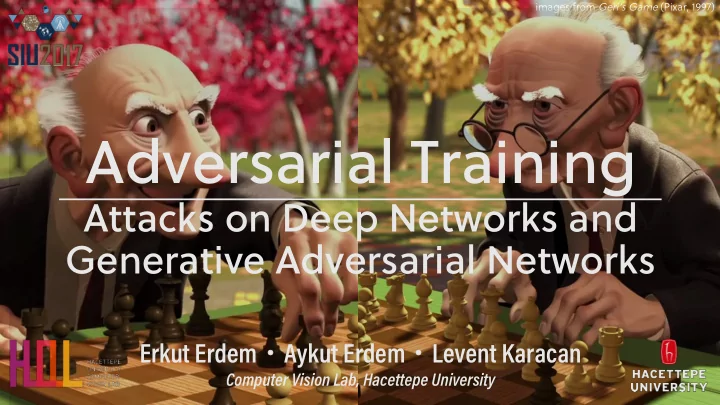
images from Geri’s Game (Pixar, 1997) Adversarial Training Attacks on Deep Networks and Generative Adversarial Networks Erkut Erdem � Aykut Erdem � Levent Karacan Computer Vision Lab, Hacettepe University

Outline • Part 1: Attacks on Deep Networks • Part 2: Generative Adversarial Networks (GANs) 10 Minutes Break • Part 3: Image Editing with GANs 2

John Carpenter’s The Thing (1982) Part 1 – Attacks on Deep Networks Erkut Erdem Computer Vision Lab, Hacettepe University

Deep Convolutional Networks in 10 mins 4

1 st Era (1940’s-1960’s): Invention • Connectionism (Hebb 1940’s) : complex behaviors arise from interconnected networks of simple units • Artificial neurons (Hebb, McCulloch and Pitts 1940’s-1950’s) • Perceptron (Rosenblatt 1950’s) : Single layer with learning rule linear 
 weighting non-linear 
 1 b accumulation activation w 1 x 1 w 2 Σ S P( y = 1 | x , w , b) x 2 w D ⁞ x D 5 Slide adapted from Rob Fergus

2 nd Era (1980’s-1990’s): Multi-layered Networks • Back-propagation (Rumelhart, Hinton and Williams 1986 +others) : effective way to train multi-layered networks • Convolutional networks (LeCun et al. 1989) : architecture adapted for images (inspired by Hubel and Wiesel’s simple/complex cells) C3: f. maps 16@10x10 C1: feature maps S4: f. maps 16@5x5 INPUT 6@28x28 32x32 S2: f. maps C5: layer OUTPUT F6: layer 6@14x14 120 10 84 Gaussian connections Full connection Subsampling Subsampling Full connection Convolutions Convolutions 6 Slide adapted from Rob Fergus

The Deep Learning Era (2011-present) • Big gains in performance on perceptual tasks: • Vision • Speech understanding • Natural language processing • Three ingredients: 1. Deep neural network models (supervised training) 2. Big labeled datasets 3. Fast GPU computation 7 Slide credit: Rob Fergus

Powerful Hardware • Deep neural nets highly amenable to implementation on Graphics Processing Units (GPUs) • Matrix multiplication • 2D convolution • Latest generation nVidia GPUs (Pascal) deliver 10 Tflops • Faster than fastest computer in the world in 2000 • 10 million times faster than 1980’s Sun workstation 8 Slide adapted from Rob Fergus

AlexNet: The Model That Changed The History • Krizhevsky, Sutskever and Hinton (2012) − 8 layer Convolutional network model [LeCun et al. 1989] − 7 hidden layers, 650,000 neurons, ~60,000,000 parameters − Trained on 1.2 million ImageNet images (with labels) − GPU implementation (50x speedup over CPU) − Training time: 1 week on pair of GPUs 9 [AlexNet by Krizhevsky et al. 2012]

Supervised Learning: Image Classification “Cat” Joshua Drewe 10

Supervised Learning: Image Classification “Cat” Model [parameters θ] Training: Adjust model parameters θ so predicted labels match true labels across training set Joshua Drewe 11

Modern Convolutional Nets [AlexNet by Krizhevsky et al. 2012] [AlexNet by Krizhevsky et al. 2012] Excellent performance in most image Millions of parameters learned from data understanding tasks The “ meaning ” of the representation is Learn a sequence of general-purpose unclear representations 12 Slide credit: Andrea Vedaldi


 Convolutions with Filters • Each filter acts on multiple input channels F − Convolution is local Filters look locally Σ Parameter sharing − Translation invariant x y Filters act the same everywhere 1 lattice 
 multiple 
 b structure feature channels f 1 x 1 f 2 Σ S x 2 F q Σ F q Σ f D ⁞ x D 13 Slide credit: Andrea Vedaldi

Convolution • Convolution = Spatial filtering • Different filters (weights) reveal a different characteristics of the input. 1 0 0 1/8 ∗ 4 1 1 0 1 0 14

Convolution • Convolution = Spatial filtering • Different filters (weights) reveal a different characteristics of the input. -1 0 0 ∗ 4 -1 -1 0 -1 0 15

Convolution • Convolution = Spatial filtering • Different filters (weights) reveal a different characteristics of the input. 0 -1 1 ∗ 0 2 -2 1 0 -1 16

Convolutional Layer • Multiple filters produce multiple output channels • For example, if we had 6 5x5 filters, we’ll get 6 separate activation maps: activation maps 32 28 Convolutional Layer 28 32 3 6 We stack these up to get an output of size 28x28x6. 17 Slide credit: Alex Karpathy

Pooling Layer • makes the representations smaller and more manageable • operates over each activation map independently: • Max pooling, average pooling, etc. Single depth slice x 1 1 2 4 max pool with 2x2 5 6 7 8 filters and stride 2 6 8 3 2 1 0 3 4 1 2 3 4 y 18 Slide adapted from Alex Karpathy

Fully Connected Layer • contains neurons that connect to the entire input volume, as in ordinary Neural Networks 19 20 Slide credit: Alex Karpathy

Feature Learning • Hierarchical layer structure allows to learn hierarchical filters (features). 20 Slide credit: Yann LeCun

Visualizing The Representation t-SNE visualization (van der Maaten & Hinton) • Embed high-dimensional points so that locally, pairwise distances are conserved • i.e. similar things end up in similar places. dissimilar things end up wherever • Right : Example embedding of MNIST digits (0-9) in 2D 21 Slide credit: Alex Karpathy

Three Years of Progress • • • AlexNet, 8 layers • rs 3x3 conv, 64 11x11 conv, 96, /4, pool/2 GoogLeNet, VGG, 19 layers softmax2 Soft maxActivat ion • 5x5 conv, 256, pool/2 3x3 conv, 64, pool/2 22 layers FC (ILSVRC 2012) AveragePool • 7x7+ 1(V) (ILSVRC 2014) s 3x3 conv, 384 3x3 conv, 128 DepthConcat Conv Conv Conv Conv • (ILSVRC 2014) 1x1+ 1(S) 3x3+ 1(S) 5x5+ 1(S) 1x1+ 1(S) 3x3 conv, 384 3x3 conv, 128, pool/2 Conv Conv MaxPool 1x1+ 1(S) 1x1+ 1(S) 3x3+ 1(S) • DepthConcat Conv Conv Conv Conv 3x3 conv, 256, pool/2 3x3 conv, 256 softmax1 1x1+ 1(S) 3x3+ 1(S) 5x5+ 1(S) 1x1+ 1(S) Conv Conv MaxPool SoftmaxActivation 1x1+ 1(S) 1x1+ 1(S) 3x3+ 1(S) • fc, 4096 3x3 conv, 256 MaxPool FC 3x3+ 2(S) DepthConcat FC • fc, 4096 3x3 conv, 256 Conv Conv Conv Conv Conv 1x1+ 1(S) 3x3+ 1(S) 5x5+ 1(S) 1x1+ 1(S) 1x1+ 1(S) Conv Conv MaxPool AveragePool 1x1+ 1(S) 1x1+ 1(S) 3x3+ 1(S) • 5x5+ 3(V) fc, 1000 3x3 conv, 256, pool/2 DepthConcat • Conv Conv Conv Conv 1x1+ 1(S) 3x3+ 1(S) 5x5+ 1(S) 1x1+ 1(S) 3x3 conv, 512 Conv Conv MaxPool 1x1+ 1(S) 1x1+ 1(S) 3x3+ 1(S) • DepthConcat softmax0 3x3 conv, 512 Conv Conv Conv Conv • SoftmaxActivation 1x1+ 1(S) 3x3+ 1(S) 5x5+ 1(S) 1x1+ 1(S) Conv Conv MaxPool FC 1x1+ 1(S) 1x1+ 1(S) 3x3+ 1(S) 3x3 conv, 512 DepthConcat FC Conv Conv Conv Conv Conv 1x1+ 1(S) 3x3+ 1(S) 5x5+ 1(S) • 1x1+ 1(S) 1x1+ 1(S) 3x3 conv, 512, pool/2 Conv Conv MaxPool AveragePool 1x1+ 1(S) 1x1+ 1(S) 3x3+ 1(S) 5x5+ 3(V) • DepthConcat 3x3 conv, 512 Conv Conv Conv Conv 1x1+ 1(S) 3x3+ 1(S) 5x5+ 1(S) 1x1+ 1(S) • Conv Conv MaxPool 1x1+ 1(S) 1x1+ 1(S) 3x3+ 1(S) 3x3 conv, 512 • Very deep • Branching MaxPool 3x3+ 2(S) • DepthConcat 3x3 conv, 512 Conv Conv Conv Conv • 1x1+ 1(S) 3x3+ 1(S) 5x5+ 1(S) 1x1+ 1(S) p g Conv Conv MaxPool 1x1+ 1(S) 1x1+ 1(S) 3x3+ 1(S) • Simply deep • Bottleneck 3x3 conv, 512, pool/2 DepthConcat ck Conv Conv Conv Conv 1x1+ 1(S) 3x3+ 1(S) 5x5+ 1(S) 1x1+ 1(S) fc, 4096 Conv Conv MaxPool 1x1+ 1(S) 1x1+ 1(S) 3x3+ 1(S) MaxPool nnection 3x3+ 2(S) • Skip connection fc, 4096 LocalRespNorm Conv 3x3+ 1(S) fc, 1000 Conv 1x1+ 1(V) , Shaoqing Ren, & Jian S LocalRespNorm MaxPool 3x3+ 2(S) 22 Conv 7x7+ 2(S) input Image Recognition”. CVP

Training Deep Neural Networks • The network is trained by stochastic gradient descent. • Backpropagation is used similarly as in a fully connected network. • Pass gradients through element-wise activation function. • We also need to pass gradients through the convolution operation and the pooling operation. 23

Object Detection Networks ImageNet detection data data backbone classification detection structure network network pre-train features fine-tune R-CNN • AlexNet • Fast R-CNN • VGG-16 • Faster R-CNN • GoogleNet • MultiBox • ResNet-101 • SSD • … • … • independently independently “plug-in” “plug-in” “plug-in” developed developed detectors feature detectors features feature 24 Slide credit: Kaiming He

ResNet’s Object Detection Results on COCO Kaiming He, Xiangyu Zhang, Shaoqing Ren, & Jian Sun. Deep Residual Learning for Image Recognition. CVPR 2016. Shaoqing Ren, Kaiming He, Ross Girshick, & Jian Sun. Faster R- CNN: Towards Real-Time Object Detection with Region Proposal Networks. NIPS 2015. 26 Slide credit: Kaiming He

ResNet’s Object Detection Results on COCO Kaiming He, Xiangyu Zhang, Shaoqing Ren, & Jian Sun. Deep Residual Learning for Image Recognition. CVPR 2016. Shaoqing Ren, Kaiming He, Ross Girshick, & Jian Sun. Faster R- CNN: Towards Real-Time Object Detection with Region Proposal Networks. NIPS 2015. 27 Slide credit: Kaiming He *the ori

Story isn't over yet! 27

Story isn't over yet! … we have reached the point where ML works, but let’s see how it can be easily fooled. 28

Adversarial Examples 29