Robust Adjusted Likelihood Function for Image Analysis Rong Duan, - PowerPoint PPT Presentation
Robust Adjusted Likelihood Function for Image Analysis Rong Duan, Wei Jiang, Hong Man Department of Electrical and Computer Engineering Stevens Institute of Technology Outline Objective: study parametric classification method when model
Robust Adjusted Likelihood Function for Image Analysis Rong Duan, Wei Jiang, Hong Man Department of Electrical and Computer Engineering Stevens Institute of Technology
Outline • Objective: study parametric classification method when model is misspecified • Method: robust adjusted likelihood function (RAL ) • Contents: 1. Likelihood function under true model 2. Model misspecification 3. Robust adjusted likelihood function 4. Simulation and application experiment 5. Conclusion
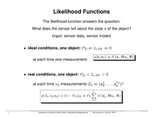
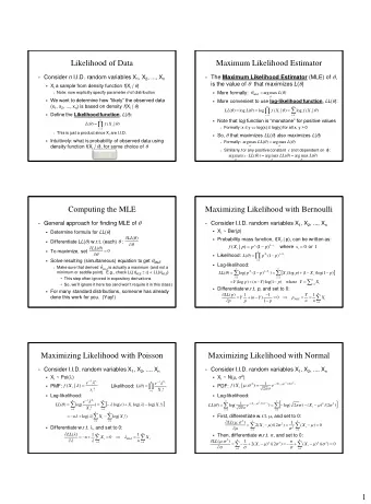
Likelihood • Let x 1 , …x n be independent random variables with pdf f ( x i ; θ ) – the likelihood function is defined as the joint density of n independent observations X =( x 1 , …, x n ) ’ ∏ n θ = θ = θ f X ( ; ) f x ( ; ) L ( ; X ) i = i 1 – the log form is = ∑ n θ θ log( ( ; L X )) log( ( f x ; )) i = i 1
Likelihood • The Law of Likelihood (Hacking 1965) – If one hypothesis H 1 , implies that a random variable X takes the value x with probability f 1 ( x ) , while other hypothesis H 2 , implies that the probability is f 2 ( x ) , then the observation X=x is evidence supporting H 1 over H 2 if f 1 ( x ) >f 2 ( x ) , and the likelihood ratio, f 1 ( x ) /f 2 ( x ) , measures the strength of that evidence
Classification • Binary classification problem: two classes of data { X 1 } = { x 1 (1) , …, x n (1) } and { X 2 }={ x 1 (2) ,…, x n (2) } from two distributions g 1 ( x ) and g 2 ( x ), where g 1 ( x ) and g 2 ( x ) are true distributions. We denote l ( x, g 2 : g 1 ) = g 2 ( x ) /g 1 ( x ) the true likelihood ratio statistic when the data x comes from the true model. • If the loss function is symmetric and the prior probabilities q ( θ k ) are equal { q θ 1 = …= q θ k } , the Bayes classifier can be expressed as a maximum likelihood test = f x θ i ' argmaxlog( ( , )) i i
Classification • The decision boundary is l ( x, θ 1 ) = l ( x, θ 2 ) , where l ( x, θ i ) =log f ( x, θ i ) • When the model assumption is correct, The Bayes classifier is optimum, it has the minimum error rate. • The distribution parameters, θ i , can be learned from training data using maximum likelihood estimation (MLE). However certain estimation error will be introduced, and estimated parameters are denoted as ˆ θ i
Model Misspecification • When the model assumption is incorrect, the maximum likelihood test will yield inferior classification results – The estimated model parameters may be erroneous – The distribution of the likelihood ratio statistic is no longer chi-square due to the failure of Bartlett's second identity
Model Misspecification • A model misspecification example: – True model: g 1 ( x ), g 2 ( x ); assumed models: f 1 ( x ), f 2 ( x )
Robust Adjustment of Likelihood • Stafford (1996) proposed a robust adjustment of likelihood function in the scalar random variable case, f ξ ( x, θ ) =f ( x, θ ) ξ • The intention is to correct the Bartlett's second identity, which equates the variance of the Fisher score θ = θ θ T J ( ) E u [ ( ; X u ) ( ; X )] g and the expected Fisher information matrix 2 log( ( )) ⎡ ⎤ ∂ θ L θ = − H ( ) E ⎢ ⎥ g ∂ ∂ θ θ T ⎣ ⎦ • Analytical expressions for calculating the parameter, ξ , are only available for a very few distributions.
Robust Adjusted Likelihood Function • We propose a general robust adjusted likelihood (RAL) function f a ( x, θ ) = η f ( x, θ ) ξ • The RAL classification rule becomes i' = arg max { log ( η ) + ξ log ( f i ( X, θ i ))} • The classification boundary is b + w l ( x, θ 1 ) = l ( x, θ 2 ), where b = { log ( η 1 )- log ( η 2 )}/ ξ 2 and w = ξ 1 / ξ 2 , this classification boundary is in a form of a linear discriminant function in likelihood space.
Robust Adjusted Likelihood Function • The RAL introduces a data-driven linear discrimination rule b + w l ( x, θ 1 ) = l ( x, θ 2 ) , where w and b are learned from training data. – If w= 1, the discrimination rule is similar to likelihood ratio tests whose evidence is controlled by the bump function if the parametric family includes g k ( x ). – If w= 1 and b= 0 , it reduces to the Bayes classification rule in the data space • A major advantage of the RAL is that its classification rule includes the Bayes classification rule as a special case. Therefore, similar to likelihood space classification, RAL will not perform worse than Bayes classification.
Minimum Error Rate Learning • Likelihood space minimum error rate learning method to estimate ( b,w ): For two classes of training data, X 1 and X 2 , – = θ − θ > ( , b w ) argmin{ P ( ( l X , ) wl X ( , ) b ) g 1 2 1 1 1 + θ − θ < P ( ( l X , ) wl X ( , ) b )} g 2 1 2 2 2 – Algorithm: 1. Initialize w 1 minimizing error rate for X 1 , i.e. e 1 , and w 2 minimizing error rate for X 2 , i.e. e 2 . Assuming w 1 > w 2 . Calculate total error rate e = e 1 + e 2 2. If w 1 ≤ w 2 or e is minimized, w =( w 1 + w 2 )/2 , stop 3. Else, decrease w 1 and increase w 2 to calculate new error rate e = e 1 + e 2 , goto step 2
Minimum Error Rate Learning
RAL Classification • RAL classification algorithm – Training: 1.Make model assumption 2.Estimate model parameters θ based on maximum likelihood method 3.Estimate RAL parameter ( b,w ) based on minimum error rate method – Testing: 1.Calculate RAL of an input sample y , 2.Classify this sample based on the maximum RAL rule.
Study on Simulated Data • Experiment: 1. Two classes data are from two Rayleigh distributions with same scale and different locations. The assumed models are Gaussian distributions with same variance. 2. The Bayes error rate of the true model, the Bayes error rate of the misspecified model, and the error rate of the robust adjusted likelihood classification are compared 3. Repeat 100 times to get the average
Study on Simulated Data
Study on Simulated Data
Application on SAR ATR • Experiment: – MSTAR SAR dataset: T72, BMP2 – Assumed models: 2 Gaussian Mixture Models (GMM) with 10 mixtures for each class. – Classification performance obtained for various training data sizes, with an increase of 10 samples each time. • Observation: – Under a practical situation, accurate model assumption is difficult to obtain, and RAL classification has an advantage to provide certain robustness in parametric classification.
Application on SAR ATR
Conclusion • The RAL classification is robust in classification when model assumption is not correct. • Minimum error rate method is effective in estimating the raising power and scale parameters from training data • In theory, RAL will not perform worse than the Bayes classifier. • Further investigation is needed to obtain theoretical performance bound for RAL under various practical situations
Recommend
More recommend
Explore More Topics
Stay informed with curated content and fresh updates.
