Passive Learning (Ch. 21.1-21.2) Step 1. EM Algorithm For an - PowerPoint PPT Presentation
Passive Learning (Ch. 21.1-21.2) Step 1. EM Algorithm For an example, lets go back to the original data but convert for hidden: P(mood) = 0.5 mood HW? P(HW=easy | mood) = 0.8 P(HW=easy | mood) = 0.25 ... saw 3 HW: easy, easy, hard
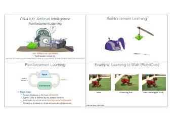
Passive Learning (Ch. 21.1-21.2)
Step 1. EM Algorithm For an example, let’s go back to the original data but convert for hidden: P(mood) = 0.5 mood HW? P(HW=easy | mood) = 0.8 P(HW=easy | ⌐mood) = 0.25 ... saw 3 HW: easy, easy, hard Step 1. is done (initialize parameter guess as the above probabilities)
Step 2. EM Algorithm Step 2: estimate unknown mood HW? In other words we need to find P(mood|data) In the case where all variables were visible, this would just have been: [number of positive mood] / total However, since we can’t see which ones, we have to estimate using parameters
Step 2. EM Algorithm If “N” is our total, then we let “ ” be our estimate count, where: (Bayes rule) So in our 2 easy, 1 difficult example: just Bayes rule: P(A|B) = P(A,B)/P(B) So our new estimate is 1/N that or: =P(B|A)P(A)/[P(A,B) + P(~A,B)] ... A=mood, B=HW more easy HW estimate I’m in a good mood
Step 3. EM Algorithm Step 3: find best parameters Now that we have P(mood) estimate, we use it to compute table for P(HW? | mood) Again, we have to approximate the number of homework that came from good/bad mood: (same as before, but don’t include “hards”)
Step 3. EM Algorithm So before we used this to calculate the total number of stuff caused by a good “mood”: Now if we want to find a new estimate for number of easy homeworks caused by mood, ignore the hard part
Step 3. EM Algorithm So before we used this to calculate the total number of stuff caused by a good “mood”: 0 Now if we want to find a new estimate for number of easy homeworks caused by mood, ignore the hard part
Step 3. EM Algorithm This means we estimate 1.523 of the “easy” HW came from a good mood We just estimated that P(mood) = 0.5781, so with 3 examples “mood” happens 1.734 (same number as original sum) an increase from our original 0.8 Thus: P(hw=easy|mood) like P(easy|mood) = P(easy,mood)/P(mood)
Step 4. EM Algorithm Then we go off and do a similar equation to get a new estimate for P(HW=easy | ⌐mood) After that, we just iterate the process, so with new value recompute P(mood) Recompute: P(HW=easy | mood) and P(HW=easy | ⌐mood) using new P(mood) Re-recompute: P(mood)...
EM Algorithm You can also use the EM algorithm on HMMs, but you have to group together all transitions (since they use the same probability) The EM algorithm is also not limited to just all things Bayesian, and can be generalized: step 3. maximize outcomes step 2. assume parameters, θ
EM Algorithm The EM algorithm is a form of gradient descent (or hill-climbing, but no α) Real distribution Some samples EM algorithm reverse-eng.
Reinforcement Learning So far we have had labeled outputs for our data (i.e. we knew the homework was easy) We will move from this (supervised learning) to where we don’t know the correct answer, just if it was good/bad (reinforcement) This is much more useful in practice as for hard problems we often don’t know the correct answer (else why’d we ask the computer?)
Reinforcement Learning We will start by looking at passive learning, where we will not be taking actions, but just observing outcomes (because easier) Next time we will move into active learning, where we can choose how we want to act to find the best outcomes/learn quickly For now we want something we can observe, but see outcomes (i.e. rewards) for actions
Reinforcement Learning To do this, we will go back to our friend MDP T T However since this is passive learning, we will only use the actions/arrows shown (T’s are terminal states, so no actions)
Reinforcement Learning How is this different than before? (1) Rewards of states not known (2) Transition function not known (i.e. no 80%, 10%, 10%) Instead we will see examples T of the MDP being run and learn the utilities T
Reinforcement Learning Suppose we start in bottom row, left-most column and take the path shown This will be recorded as (state) reward : 1 2 3 4 (4,2) -1 ↑(3,2) -1 →(4,2) -1 T 1 ↑(3,2) -1 →(2,2) -1 ↑(1,2) 50 2 3 T ... then repeat this for more 4 examples to better learn
Direct Utility Estimation (4,2) -1 ↑(3,2) -1 →(4,2) -1 ↑(3,2) -1 →(2,2) -1 ↑(1,2) 50 The first (of three) ways to do passive learning is called direct utility estimation using reward: assume γ=1 for simplicity Given this sequence, we can calculate the rewards at each step (starting from end): (1,2) has reward 50-1-1-1-1-1=45 Then (2,2) is one more, so 45+1 = 46... so on
Direct Utility Estimation This gives us: (4,2) -1 ↑(3,2) -1 →(4,2) -1 ↑(3,2) -1 →(2,2) -1 ↑(1,2) 50 40 41 42 43 44 45 Then we just find the average reward (4,2) visited twice (40,42)... average = 41 ... and so on (1,2) visited once... average reward = 45 Then update averages with future examples
Direct Utility Estimation So let’s say you go straight to goal: (4,2) -1 ↑(3,2) -1 →(2,2) -1 ↑(1,2) 50 44 45 46 47 Then we update old averages with new data (only need store counts): (4,2) visited once (44)... new average = 44 (1,2) visited once... new average = 47, so running total average now (45+47)/2=46
Direct Utility Estimation Given that we are sampling the actions, this should lead to the correct expected rewards just by simple average (This also has changed problem back to supervised, as we “see” outcomes of actions) But we can speed this up (i.e. learn much faster) by using some information What info have we not used?
Adaptive Dynamic Prog. We didn’t include our bud Bellman! no max over actions (a), as in passive actions are fixed Thus, if we can learn the rewards and transitions, we can use our normal ways of solving MDPs (value/policy iteration) This is useful as we can combine information across different states for faster learning
Adaptive Dynamic Prog. So given the same first example: (4,2) -1 ↑(3,2) -1 →(4,2) -1 ↑(3,2) -1 →(2,2) -1 ↑(1,2) 50 We’d estimate the following transitions: (4,2) + ↑ = 100% ↑ (2 of 2) (3,2) + → = 50% ↑, 50% ↓ (2,2) + ↑ = 100% ↑ ... and we can easily see the rewards from sequence, so policy/value iteration time! better as actions fixed no iteration
Adaptive Dynamic Prog. This method is called adaptive dynamic programming Using the relationship between utilities (i.e. neighbors cannot change too much) allows us to learn quicker This can be sped up even more if we assume all actions have the same outcome (i.e. going “up” has same probability for any state)
Temporal-Difference The third (last) way of doing passive learning is temporal-difference learning temporal = “time” This is a combination of the first two methods, we will keep a “running average” of each state’s utility, but also use Bellman equation Instead of directly averaging rewards to find utility, we will incrementally adjust them using the Bellman equation
Temporal-Difference Suppose we saw this example (bit different): (4,2) -1 ↑(3,2) -1 →(2,2) -1 ↑(3,2) -1 →(2,2) -1 ↑(1,2) 50 Using the direct averaging we would get: U(4,2) = 40, U(3,2) = 42 However the sample(s) so far: (4,2)↑ is always (3,2), so we’d expect (from Bellman):
Temporal-Difference This would indicate our guess of U(4,2)=40 is a bit low (or U(3,2) is a bit high) So instead of direct average, we will do incremental adjustments using Bellman: learning rate/constant So whenever you take an action, you update the utility of the state before the action (final terminal state does not need updating)
Temporal-Difference Let’s continue our example: (4,2) -1 ↑(3,2) -1 →(2,2) -1 ↑(3,2) -1 →(2,2) -1 ↑(1,2) 50 So from first example: U(4,2)=40, U(3,2)=42 If second example starts as: could use TD learning on (4,2) -1 ↑(3,2) -1 →... first example too... new states have U(s) = R(s), then do updates as described We’d update (4,2) as: (assume α=0.5)
Recap: Passive Learning What are pros/cons between the last two methods? (adapt. dyn. prog. vs temporal-diff.) Which do you think is faster at learning in general?
Recap: Passive Learning What are pros/cons between the last two methods? (adapt. dyn. prog. vs temporal-diff.) -Temporal-difference only changes a single value for each action seen -ADP would re-solve a system of linear equations (policy “iteration”) for each action Which do you think is faster at learning in general? As ADP uses Bellman equations/constraints in full it learns better (but more computation)
Recap: Passive Learning From the book’s example: ADP TD
Recommend
More recommend
Explore More Topics
Stay informed with curated content and fresh updates.

