Reinforcement Learning January 28, 2010 CS 886 University of - PowerPoint PPT Presentation
Reinforcement Learning January 28, 2010 CS 886 University of Waterloo Outline Russell & Norvig Sect 21.1-21.3 What is reinforcement learning Temporal-Difference learning Q-learning 2 CS886 Lecture Slides (c) 2010 K.
Reinforcement Learning January 28, 2010 CS 886 University of Waterloo
Outline • Russell & Norvig Sect 21.1-21.3 • What is reinforcement learning • Temporal-Difference learning • Q-learning 2 CS886 Lecture Slides (c) 2010 K. Larson and P. Poupart
Machine Learning • Supervised Learning – Teacher tells learner what to remember • Reinforcement Learning – Environment provides hints to learner • Unsupervised Learning – Learner discovers on its own 3 CS886 Lecture Slides (c) 2010 K. Larson and P. Poupart
What is RL? • Reinforcement learning is learning what to do so as to maximize a numerical reward signal – Learner is not told what actions to take, but must discover them by trying them out and seeing what the reward is 4 CS886 Lecture Slides (c) 2010 K. Larson and P. Poupart
What is RL • Reinforcement learning differs from supervised learning Reinforcement learning Supervised learning Don’t touch. You will get burnt Ouch! 5 CS886 Lecture Slides (c) 2010 K. Larson and P. Poupart
Animal Psychology • Negative reinforcements: – Pain and hunger • Positive reinforcements: – Pleasure and food • Reinforcements used to train animals • Let’s do the same with computers! 6 CS886 Lecture Slides (c) 2010 K. Larson and P. Poupart
RL Examples • Game playing (backgammon, solitaire) • Operations research (pricing, vehicule routing) • Elevator scheduling • Helicopter control • http://neuromancer.eecs.umich.edu/cgi- bin/twiki/view/Main/SuccessesOfRL 7 CS886 Lecture Slides (c) 2010 K. Larson and P. Poupart
Reinforcement Learning • Definition: – Markov decision process with unknown transition and reward models • Set of states S • Set of actions A – Actions may be stochastic • Set of reinforcement signals (rewards) – Rewards may be delayed 8 CS886 Lecture Slides (c) 2010 K. Larson and P. Poupart
Policy optimization • Markov Decision Process: – Find optimal policy given transition and reward model – Execute policy found • Reinforcement learning: – Learn an optimal policy while interacting with the environment 9 CS886 Lecture Slides (c) 2010 K. Larson and P. Poupart
Reinforcement Learning Problem Agent State Action Reward Environment a0 a1 a2 … s0 s1 s2 r1 r2 r0 Goal: Learn to choose actions that maximize r 0 + γ r 1 + γ 2 r 2 +…, where 0· γ <1 10 CS886 Lecture Slides (c) 2010 K. Larson and P. Poupart
Example: Inverted Pendulum • State: x(t),x’(t), θ (t), θ ’(t) • Action: Force F • Reward: 1 for any step where pole balanced Problem: Find δ :S → A that maximizes rewards 11 CS886 Lecture Slides (c) 2010 K. Larson and P. Poupart
Rl Characterisitics • Reinforcements: rewards • Temporal credit assignment: when a reward is received, which action should be credited? • Exploration/exploitation tradeoff: as agent learns, should it exploit its current knowledge to maximize rewards or explore to refine its knowledge? • Lifelong learning: reinforcement learning 12 CS886 Lecture Slides (c) 2010 K. Larson and P. Poupart
Types of RL • Passive vs Active learning – Passive learning: the agent executes a fixed policy and tries to evaluate it – Active learning: the agent updates its policy as it learns • Model based vs model free – Model-based: learn transition and reward model and use it to determine optimal policy – Model free: derive optimal policy without learning the model 13 CS886 Lecture Slides (c) 2010 K. Larson and P. Poupart
Passive Learning • Transition and reward model known: – Evaluate δ : – V δ (s) = R(s) + γ Σ s’ Pr(s’|s, δ (s)) V δ (s’) • Transition and reward model unknown: – Estimate policy value as agent executes policy: V δ (s) = E δ [ Σ t γ t R(s t )] – Model based vs model free 14 CS886 Lecture Slides (c) 2010 K. Larson and P. Poupart
Passive learning r r r +1 3 γ = 1 u u -1 2 r i = -0.04 for non-terminal states u l l l 1 Do not know the transition 1 2 3 4 probabilities (1,1) � (1,2) � (1,3) � (1,2) � (1,3) � (2,3) � (3,3) � (4,3) +1 (1,1) � (1,2) � (1,3) � (2,3) � (3,3) � (3,2) � (3,3) � (4,3) +1 (1,1) � (2,1) � (3,1) � (3,2) � (4,2) -1 What is the value V(s) of being in state s? 15 CS886 Lecture Slides (c) 2010 K. Larson and P. Poupart
Passive ADP • Adaptive dynamic programming (ADP) – Model-based – Learn transition probabilities and rewards from observations – Then update the values of the states 16 CS886 Lecture Slides (c) 2010 K. Larson and P. Poupart
ADP Example γ = 1 r r r +1 r i = -0.04 for non-terminal states 3 u u -1 2 V δ (s) = R(s) + γ Σ s’ Pr(s’|s, δ (s)) V δ (s’) u l l l 1 1 2 3 4 (1,1) � (1,2) � (1,3) � (1,2) � (1,3) � (2,3) � (3,3) � (4,3) +1 (1,1) � (1,2) � (1,3) � (2,3) � (3,3) � (3,2) � (3,3) � (4,3) +1 (1,1) � (2,1) � (3,1) � (3,2) � (4,2) -1 P((2,3)|(1,3),r) =2/3 Use this information in P((1,2)|(1,3),r) =1/3 We need to learn all the transition probabilities! 17 CS886 Lecture Slides (c) 2010 K. Larson and P. Poupart
Passive TD • Temporal difference (TD) – Model free • At each time step – Observe: s,a,s’,r – Update V δ (s) after each move – V δ (s) = V δ (s) + α (R(s) + γ V δ (s’) – V δ (s)) Learning rate Temporal difference 18 CS886 Lecture Slides (c) 2010 K. Larson and P. Poupart
TD Convergence Thm: If α is appropriately decreased with number of times a state is visited then V δ (s) converges to correct value • α must satisfy: • Σ t α t � ∞ • Σ t ( α t ) 2 < ∞ • Often α (s) = 1/n(s) • n(s) = # of times s is visited 19 CS886 Lecture Slides (c) 2010 K. Larson and P. Poupart
Active Learning • Ultimately, we are interested in improving δ • Transition and reward model known: – V * (s) = max a R(s) + γ Σ s’ Pr(s’|s,a) V * (s’) • Transition and reward model unknown: – Improve policy as agent executes policy – Model based vs model free 20 CS886 Lecture Slides (c) 2010 K. Larson and P. Poupart
Q-learning (aka active temporal difference) • Q-function: Q:S × A →ℜ – Value of state-action pair – Policy δ (s) = argmax a Q(s,a) is the optimal policy • Bellman’s equation: Q*(s,a) = R(s) + γ Σ s’ Pr(s’|s,a) max a’ Q*(s’,a’) 21 CS886 Lecture Slides (c) 2010 K. Larson and P. Poupart
Q-learning • For each state s and action a initialize Q(s,a) (0 or random) • Observe current state • Loop – Select action a and execute it – Receive immediate reward r – Observe new state s’ – Update Q(s,a) • Q(s,a) = Q(s,a) + α (r(s)+ γ max a’ Q(s’,a’) – Q(s,a)) – s=s’ 22 CS886 Lecture Slides (c) 2010 K. Larson and P. Poupart
Q-learning example s 1 s 2 73 81.5 100 100 66 66 81 81 r=0 for non-terminal states γ= 0.9 α =0.5 Q(s 1 ,right) = Q(s 1 ,right) + α (r(s 1 ) + γ max a’ Q(s 2 ,a’) – Q(s 1 ,right)) = 73 + 0.5 (0 + 0.9 max[66,81,100] – 73) = 73 + 0.5 (17) = 81.5 23 CS886 Lecture Slides (c) 2010 K. Larson and P. Poupart
Q-learning • For each state s and action a initialize Q(s,a) (0 or random) • Observe current state • Loop – Select action a and execute it – Receive immediate reward r – Observe new state s’ – Update Q(a,s) • Q(s,a) = Q(s,a) + α (r(s)+ γ max a’ Q(s’,a’) – Q(s,a)) – s=s’ 24 CS886 Lecture Slides (c) 2010 K. Larson and P. Poupart
Exploration vs Exploitation • If an agent always chooses the action with the highest value then it is exploiting – The learned model is not the real model – Leads to suboptimal results • By taking random actions (pure exploration) an agent may learn the model – But what is the use of learning a complete model if parts of it are never used? • Need a balance between exploitation and exporation 25 CS886 Lecture Slides (c) 2010 K. Larson and P. Poupart
Common exploration methods • ε -greedy: – With probability ε execute random action – Otherwise execute best action a* a* = argmax a Q(s,a) • Boltzmann exploration P(a) = e Q(s,a)/T Σ a e Q(s,a)/T 26 CS886 Lecture Slides (c) 2010 K. Larson and P. Poupart
Exploration and Q-learning • Q-learning converges to optimal Q- values if – Every state is visited infinitely often (due to exploration) – The action selection becomes greedy as time approaches infinity – The learning rate a is decreased fast enough but not too fast 27 CS886 Lecture Slides (c) 2010 K. Larson and P. Poupart
A Triumph for Reinforcement Learning: TD-Gammon • Backgammon player: TD learning with a neural network representation of the value function: 28 CS886 Lecture Slides (c) 2010 K. Larson and P. Poupart
Recommend
More recommend
Explore More Topics
Stay informed with curated content and fresh updates.
