Overview of this module Course 02429 Analysis of correlated data: - PowerPoint PPT Presentation

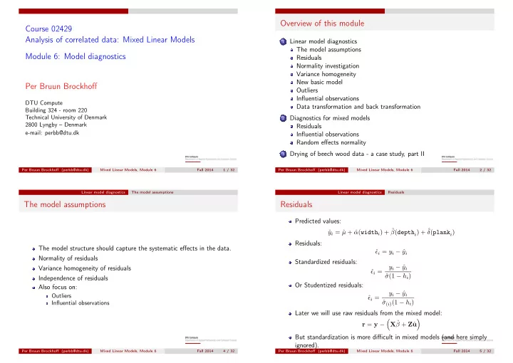
Overview of this module Course 02429 Analysis of correlated data: Mixed Linear Models Linear model diagnostics 1 The model assumptions Module 6: Model diagnostics Residuals Normality investigation Variance homogeneity New basic model Per Bruun Brockhoff Outliers Influential observations DTU Compute Data transformation and back transformation Building 324 - room 220 Technical University of Denmark Diagnostics for mixed models 2 2800 Lyngby – Denmark Residuals e-mail: perbb@dtu.dk Influential observations Random effects normality Drying of beech wood data - a case study, part II 3 Per Bruun Brockhoff (perbb@dtu.dk) Mixed Linear Models, Module 6 Fall 2014 1 / 32 Per Bruun Brockhoff (perbb@dtu.dk) Mixed Linear Models, Module 6 Fall 2014 2 / 32 Linear model diagnostics The model assumptions Linear model diagnostics Residuals The model assumptions Residuals Predicted values: α ( width i ) + ˆ β ( depth i ) + ˆ y i = ˆ ˆ µ + ˆ δ ( plank i ) Residuals: The model structure should capture the systematic effects in the data. ǫ i = y i − ˆ ˆ y i Normality of residuals Standardized residuals: y i − ˆ y i Variance homogeneity of residuals ǫ i = ˆ σ (1 − h i ) ˆ Independence of residuals Or Studentized residuals: Also focus on: y i − ˆ y i Outliers ǫ i = ˆ σ ( i ) (1 − h i ) ˆ Influential observations Later we will use raw residuals from the mixed model: � � X ˆ β + Z ˆ r = y − u But standardization is more difficult in mixed models (and here simply ignored). Per Bruun Brockhoff (perbb@dtu.dk) Mixed Linear Models, Module 6 Fall 2014 4 / 32 Per Bruun Brockhoff (perbb@dtu.dk) Mixed Linear Models, Module 6 Fall 2014 5 / 32