Kernel Based Estimation of Inequality Indices and Risk Measures - PowerPoint PPT Presentation

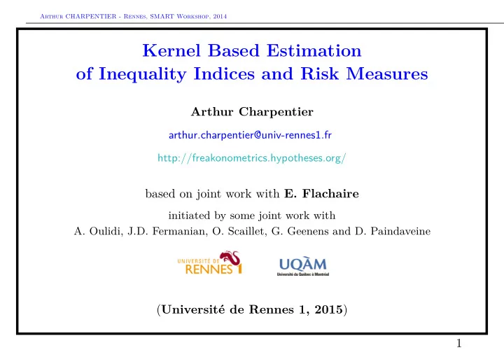
Arthur CHARPENTIER - Rennes, SMART Workshop, 2014 Kernel Based Estimation of Inequality Indices and Risk Measures Arthur Charpentier arthur.charpentier@univ-rennes1.fr http://freakonometrics.hypotheses.org/ based on joint work with E. Flachaire initiated by some joint work with A. Oulidi, J.D. Fermanian, O. Scaillet, G. Geenens and D. Paindaveine ( Université de Rennes 1, 2015 ) 1

Arthur CHARPENTIER - Rennes, SMART Workshop, 2014 Stochastic Dominance and Related Indices • First Order Stochastic Dominance (cf standard stochastic order, � st ) X � 1 Y ⇐ ⇒ F X ( t ) ≥ F Y ( t ) , ∀ t ⇐ ⇒ VaR X ( u ) ≤ VaR Y ( u ) , ∀ u • Convex Stochastic Dominance (cf martingale property) ⇒ E [ ˜ Y | ˜ X ] = ˜ X � cx Y ⇐ X ⇐ ⇒ ES X ( u ) ≤ ES Y ( u ) , ∀ u and E ( X ) = E ( Y ) • Second Order Stochastic Dominance (cf submartingale property, stop-loss order, � icx ) ⇒ E [ ˜ Y | ˜ X ] ≥ ˜ X � 2 Y ⇐ X ⇐ ⇒ ES X ( u ) ≤ ES Y ( u ) , ∀ u • Lorenz Stochastic Dominance (cf dilatation order) X X X � L Y ⇐ ⇒ E [ X ] � cx E [ Y ] ⇐ ⇒ L X ( u ) ≤ L Y ( u ) , ∀ u 2

Arthur CHARPENTIER - Rennes, SMART Workshop, 2014 Stochastic Dominance and Related Indices • Parametric Model(s) E.g. N ( µ X , σ 2 X ) � 1 N ( µ Y , σ 2 ⇒ µ X ≤ µ Y and σ 2 X = σ 2 Y ) ⇐ Y E.g. N ( µ X , σ 2 X ) � cx N ( µ Y , σ 2 ⇒ µ X = µ Y and σ 2 X ≤ σ 2 Y ) ⇐ Y E.g. N ( µ X , σ 2 X ) � 2 N ( µ Y , σ 2 ⇒ µ X ≤ µ Y and σ 2 X ≤ σ 2 Y ) ⇐ Y Or other parametric distribution. E.g. a lognormal distribution for losses 0.30 1.0 0.25 0.8 0.20 Cumulated Density 0.6 Density 0.15 0.4 0.10 0.2 0.05 0.00 0.0 0 5 10 15 20 25 0 5 10 15 20 25 3

Arthur CHARPENTIER - Rennes, SMART Workshop, 2014 Stochastic Dominance and Related Indices • Non-parametric Model(s) 0.30 1.0 0.25 0.8 0.20 Cumulated Density 0.6 Density 0.15 0.4 0.10 0.2 0.05 0.00 0.0 0 5 10 15 20 25 0 5 10 15 20 25 4

Arthur CHARPENTIER - Rennes, SMART Workshop, 2014 Nonparametric estimation of the density 0.6 0.5 0.4 density 0.3 0.2 0.1 0.0 0 20 40 60 80 5

Arthur CHARPENTIER - Rennes, SMART Workshop, 2014 Agenda F n ( · ) or � � F − 1 n ( · ) ր � sample { y 1 , · · · , y n } − → f n ( · ) ց R ( � f n ) • Estimating densities of copulas ◦ Beta kernels ◦ Transformed kernels • Combining transformed and Beta kernels • Moving around the Beta distribution ◦ Mixtures of Beta distributions ◦ Bernstein Polynomials • Some probit type transformations 6

Arthur CHARPENTIER - Rennes, SMART Workshop, 2014 Non parametric estimation of copula density see C., Fermanian & Scaillet (2005), bias of kernel estimators at endpoints Kernel based estimation of the uniform density on [0,1] Kernel based estimation of the uniform density on [0,1] 1.2 1.2 1.0 1.0 0.8 0.8 Density Density 0.6 0.6 0.4 0.4 0.2 0.2 0.0 0.0 0.0 0.2 0.4 0.6 0.8 1.0 0.0 0.2 0.4 0.6 0.8 1.0 7

Arthur CHARPENTIER - Rennes, SMART Workshop, 2014 Non parametric estimation of copula density � 1 c (0 , 0 , h )) = 1 4 · c ( u, v ) − 1 e.g. E ( � 2[ c 1 (0 , 0) + c 2 (0 , 0)] ωK ( ω ) dω · h + o ( h ) 0 Estimation of Frank copula Estimation of Frank copula 1.0 5 5 0.8 4 4 0.6 3 3 0.4 2 2 0.8 0.8 0.6 0.6 0.2 0.4 0.4 1 1 0.2 0.2 0.0 0 0 0.2 0.4 0.6 0.8 0.2 0.4 0.6 0.8 0.0 0.2 0.4 0.6 0.8 1.0 with a symmetric kernel (here a Gaussian kernel). 8

Arthur CHARPENTIER - Rennes, SMART Workshop, 2014 Non parametric estimation of copula density Standard Gaussian kernel estimator, n=100 Standard Gaussian kernel estimator, n=1000 Standard Gaussian kernel estimator, n=10000 4 4 4 3 3 3 Density of the estimator Density of the estimator Density of the estimator 2 2 2 1 1 1 0 0 0 0.0 0.2 0.4 0.6 0.8 1.0 0.0 0.2 0.4 0.6 0.8 1.0 0.0 0.2 0.4 0.6 0.8 1.0 Estimation of the density on the diagonal Estimation of the density on the diagonal Estimation of the density on the diagonal Nice asymptotic properties, see Fermanian et al. (2005)... but still: on finite sample, bad behavior on borders. 9

Arthur CHARPENTIER - Rennes, SMART Workshop, 2014 Beta kernel idea (for copulas) see Chen (1999, 2000), Bouezmarni & Rolin (2003), � � � � � � − ( u − x i ) 2 x 1 ,i x 2 ,i x 1 ,i x 2 ,i K x i ( u ) ∝ exp vs. K x i ( u ) ∝ u [1 − u 1 ] · u [1 − u 2 ] b b b b 1 2 h 2 ● ● ● ● ● ● ● ● ● ● ● ● ● ● ● ● ● ● ● ● ● ● ● ● ● ● ● ● ● ● ● ● ● ● ● ● ● ● ● ● ● ● ● ● ● ● ● ● ● ● ● ● ● ● ● ● ● ● ● ● ● ● ● ● ● ● ● ● ● ● ● ● ● ● ● ● ● ● ● ● ● ● ● ● ● ● ● ● ● ● ● ● ● ● ● ● ● ● ● ● ● ● ● ● ● ● ● ● ● ● ● ● ● ● ● ● ● ● ● ● ● ● ● ● ● ● ● ● ● ● ● ● ● ● ● ● ● ● ● ● ● ● ● ● ● ● ● ● ● ● ● ● ● ● ● ● ● ● ● ● ● ● ● ● ● ● ● ● ● ● ● ● ● ● ● ● ● ● ● ● ● ● ● ● ● ● ● ● ● ● ● ● ● ● ● ● ● ● ● ● ● ● ● ● ● ● ● ● ● ● ● ● ● ● ● ● ● ● ● ● ● ● ● ● ● ● ● ● ● ● ● ● ● ● ● ● ● ● ● ● ● ● ● ● ● ● ● ● ● ● ● ● ● ● ● ● ● ● ● ● ● ● ● ● ● ● ● ● ● ● ● ● ● ● ● ● ● ● ● ● ● ● ● ● ● ● ● ● ● ● ● ● ● ● ● ● ● ● ● ● ● ● ● ● ● ● ● ● ● ● ● ● ● ● ● ● ● ● ● ● ● ● ● ● ● ● ● ● ● ● ● ● ● ● ● ● ● ● ● ● ● ● ● ● ● ● ● ● ● ● ● ● ● ● ● ● ● ● ● ● ● ● ● ● ● ● ● ● ● ● ● ● ● ● ● ● ● ● ● ● ● ● ● ● ● ● ● ● ● ● ● ● ● ● ● ● ● ● ● ● 10

Arthur CHARPENTIER - Rennes, SMART Workshop, 2014 Beta kernel idea (for copulas) Beta (independent) bivariate kernel , x=0.0, y=0.0 Beta (independent) bivariate kernel , x=0.2, y=0.0 Beta (independent) bivariate kernel , x=0.5, y=0.0 Beta (independent) bivariate kernel , x=0.0, y=0.2 Beta (independent) bivariate kernel , x=0.2, y=0.2 Beta (independent) bivariate kernel , x=0.5, y=0.2 Beta (independent) bivariate kernel , x=0.0, y=0.5 Beta (independent) bivariate kernel , x=0.2, y=0.5 Beta (independent) bivariate kernel , x=0.5, y=0.5 11

Arthur CHARPENTIER - Rennes, SMART Workshop, 2014 Beta kernel idea (for copulas) Estimation of Frank copula Estimation of the copula density (Beta kernel, b=0.1) Estimation of the copula density (Beta kernel, b=0.05) 5 3.0 3.0 4 2.5 2.5 3 2.0 2.0 1.5 1.5 2 0.8 0.6 0.8 0.8 1.0 1.0 0.6 0.6 0.4 1 0.4 0.4 0.5 0.5 0.2 0.2 0.2 0 0.0 0.0 0.2 0.4 0.6 0.8 0.2 0.4 0.6 0.8 0.2 0.4 0.6 0.8 12

Arthur CHARPENTIER - Rennes, SMART Workshop, 2014 Beta kernel idea (for copulas) Beta kernel estimator, b=0.05, n=100 Beta kernel estimator, b=0.02, n=1000 Beta kernel estimator, b=0.005, n=10000 4 4 4 3 3 3 Density of the estimator Density of the estimator Density of the estimator 2 2 2 1 1 1 0 0 0 0.0 0.2 0.4 0.6 0.8 1.0 0.0 0.2 0.4 0.6 0.8 1.0 0.0 0.2 0.4 0.6 0.8 1.0 Estimation of the density on the diagonal Estimation of the density on the diagonal Estimation of the density on the diagonal 13

Arthur CHARPENTIER - Rennes, SMART Workshop, 2014 Transformed kernel idea (for copulas) [0 , 1] × [0 , 1] → R × R → [0 , 1] × [0 , 1] 14

Arthur CHARPENTIER - Rennes, SMART Workshop, 2014 Transformed kernel idea (for copulas) Estimation of Frank copula Estimation of Frank copula Estimation of Frank copula 5 5 5 4 4 4 3 3 3 2 2 2 0.8 0.8 0.8 0.6 0.6 0.6 0.4 0.4 0.4 1 1 1 0.2 0.2 0.2 0 0 0 0.2 0.4 0.6 0.8 0.2 0.4 0.6 0.8 0.2 0.4 0.6 0.8 15

Arthur CHARPENTIER - Rennes, SMART Workshop, 2014 Transformed kernel idea (for copulas) Transformed kernel estimator (Gaussian), n=100 Transformed kernel estimator (Gaussian), n=1000 Transformed kernel estimator (Gaussian), n=10000 4 4 4 3 3 3 Density of the estimator Density of the estimator Density of the estimator 2 2 2 1 1 1 0 0 0 0.0 0.2 0.4 0.6 0.8 1.0 0.0 0.2 0.4 0.6 0.8 1.0 0.0 0.2 0.4 0.6 0.8 1.0 Estimation of the density on the diagonal Estimation of the density on the diagonal Estimation of the density on the diagonal see Geenens, C. & Paindaveine (2014) for more details on probit transformation for copulas. 16

Arthur CHARPENTIER - Rennes, SMART Workshop, 2014 Combining the two approaches See Devroye & Györfi (1985), and Devroye & Lugosi (2001) ... use the transformed kernel the other way, R → [0 , 1] → R 17

Arthur CHARPENTIER - Rennes, SMART Workshop, 2014 Devroye & Györfi (1985) - Devroye & Lugosi (2001) Interesting point, the optimal T should be F , thus, T can be F � θ 18