Contents 1 Introduction 1 2 Linear Transformations 2 3 - PDF document

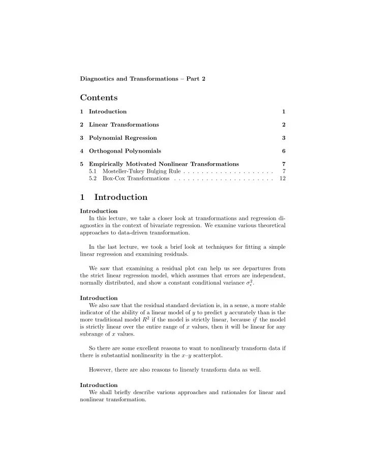
Diagnostics and Transformations – Part 2 Contents 1 Introduction 1 2 Linear Transformations 2 3 Polynomial Regression 3 4 Orthogonal Polynomials 6 5 Empirically Motivated Nonlinear Transformations 7 5.1 Mosteller-Tukey Bulging Rule . . . . . . . . . . . . . . . . . . . . 7 5.2 Box-Cox Transformations . . . . . . . . . . . . . . . . . . . . . . 12 1 Introduction Introduction In this lecture, we take a closer look at transformations and regression di- agnostics in the context of bivariate regression. We examine various theoretical approaches to data-driven transformation. In the last lecture, we took a brief look at techniques for fitting a simple linear regression and examining residuals. We saw that examining a residual plot can help us see departures from the strict linear regression model, which assumes that errors are independent, normally distributed, and show a constant conditional variance σ 2 ǫ . Introduction We also saw that the residual standard deviation is, in a sense, a more stable indicator of the ability of a linear model of y to predict y accurately than is the more traditional model R 2 if the model is strictly linear, because if the model is strictly linear over the entire range of x values, then it will be linear for any subrange of x values. So there are some excellent reasons to want to nonlinearly transform data if there is substantial nonlinearity in the x – y scatterplot. However, there are also reasons to linearly transform data as well. Introduction We shall briefly describe various approaches and rationales for linear and nonlinear transformation.

2 Linear Transformations Linear Transformations Linear transformations of variables do not affect the accuracy of prediction in linear regression. Any change in the x or y variables will be compensated for in corresponding changes in the β values. However, various linear transforms can still be important for at least 3 rea- sons: ❼ Avoiding nonsensical values ❼ Increasing comparability ❼ Reducing collinearity of predictors Avoiding Nonsensical Values by Centering Technically, in the simple linear regression equation, the y -intercept coeffi- cient b 0 is the value of y when x = 0. In many cases, x = 0 does not correspond well to physical reality, as when, for example x is a person’s height and y their weight. In such cases, it makes sense to at least center the variable x , i.e., convert it to deviation score form by subtracting its mean. After centering the heights, a value x = 0 corresponds to an average height, and so the y -intercept would be interpreted as the average weight of people who are of average height. Enhancing Comparability by Z -Score Standardization After centering variables, they can be standardized by dividing by their standard deviation, thus converting them to z -score form. When variables are in this form, their means are always 0 and their standard deviations are always 1, so differences are always on the same scale. Standardizing to a Convenient Metric Sometimes, convenience is an overriding concern, and rather then standard- izing to z -score form, you choose a metric like income in tens of thousands of dollars that allows easy intrepretability. Standardizing to a Standard Deviation of 1/2 In section 4.2, Gelman & Hill recommend standardizing numeric (not binary) “input variables”to a mean of zero and a standard deviation of 1/2, by centering, then dividing by 2 standard deviations. 2

They state that doing this “maintains coherence when considering binary input variables.” (Binary variables coded 0,1 have a standard deviation of 1/2 when p = 0 . 5. Changing from 0 to 1 implies a shift of 2 standard deviations, which in turn results in the β weight being reduced by a factor of 2.) Gelman & Hill explain the rationale very briefly, and this rationale is con- veyed in more clarity and detail in Gelman’s (2008) article in Statistics in Medicine. Standardizing to a Standard Deviation of 1/2 Recall that a β conveys how much y should will increase on average for a unit increase in x . If numeric input variables are standardized, a unit increase in x corresponds to a standard deviation. However, if binary variables are coded 0,1 a unit increase from 0 to 1 corresponds to two standard deviations. Gelman & Hill see this as cause for concern, as linear regression compensates for this by decreasing the β weights on binary variables. By decreasing the standard deviation of numeric input variables to 1/2, they seek to eliminate what they see as an inherent interpretational disadvantage for binary variables. Standardizing to a Standard Deviation of 1/2 Comment. I don’t (yet!) see this argument as particularly convincing, be- cause the standard deviation itself has meaning only in connection with a mean- ingful scale, which binary variables don’t have. Ultimately, a conviction to understand what numerical values actually mean in any data analytic context should trump attempts to automatize this process. Standardizing to Eliminate Problems in Interpreting Interactions When one of the variables is binary, and interaction effects exist, centering can substantially aid the interpretation of coefficients, because such interpreta- tions rely on a meaningful zero point. For example, if the model with coefficients is y = 14 + 34 x 1 + 12 x 2 + 14 x 1 x 2 the coefficient 34 is the amount of gain in y for unit change in x only when x 2 = 0. 3 Polynomial Regression Gelman & Hill distinguish in their terminology between input variables and predictors . A quick example: 3

Example 1 (Input Variables vs. Predictors) . Consider a single y predicted from a single x . We might write y = β 1 x + β 0 + ǫ Alternatively, we might write y = β 1 x + β 2 x 2 + β 0 + ǫ In each case, the input variable is x . In the first case, there is also only one predictor, x , while in the second case, there are two predictors, x and x 2 . In one sense, the second regression is nonlinear, because y is predicted from a nonlinear function of the input variable x . In another sense, it is linear, because y is predicted from a linear function of the predictors x and x 2 . In polynomial regression, we fit a polynomial in x of degree q to a criterion variable y . Example 2 (Degree 3 Polynomial) . For example, a polynomial regression of degree 3 would fit the model y = b 0 + b 1 x + b 2 x 2 + b 3 x 3 + ǫ Practical Limitations ❼ If we use polynomial regression, we need to limit the order of the polyno- mial ❼ Perfect fit to N data points can always be achieved with a degree N − 1 polynomial ❼ Fit always improves as we add more terms ❼ Terms are not uncorrelated, which adds to interpretation problems, al- though centering generally will reduce the correlation between polynomial terms Polynomial Regression Brett Larget at Wisconsin has a nice writeup on polynomial regression. Fol- lowing his example, let’s create some artificial polynomial data. > set.seed (12345) > x ← rnorm (20, mean = 0, sd = 1) > y ← 1 + 2 ✯ x + 3 ✯ x^2 + rnorm (20, sd = 0.5) > plot (x, y) 4

● 15 10 ● ● y 5 ● ● ● ● ● ● ● ● ● ● ● ● ● ● ● 0 ● ● −1 0 1 x Polynomial Regression Let’s fit a sequence of polynomial models to these data. Note the use of the I operator. In R’s model interpretation language, x*x has a special meaning, so you need to use this operator to convey to R that you intend an expression to be interpreted as a numerical transformation. > x ← x - mean (x) ← lm (y ˜ 1) > fit0 ← lm (y ˜ x) > fit1 ← lm (y ˜ x + I (x^2)) > fit2 ← lm (y ˜ x + I (x^2) + I (x^3)) > fit3 ← lm (y ˜ x + I (x^2) + I (x^3) + I (x^4)) > fit4 ← lm (y ˜ x + I (x^2) + I (x^3) + I (x^4) + I (x^5)) > fit5 Let’s examine the fit of these regression lines graphically : > ## start by plotting the data > plot (x,y) > ## add the line of linear fit in red > curve ( cbind (1,x) % ✯ % coef (fit1), col = ✬ red ✬ , add =TRUE) > ## and quadratic fit in black > curve ( cbind (1,x,x^2) % ✯ % coef (fit2), add =TRUE) > ## and cubic fit in blue > curve ( cbind (1,x,x^2,x^3) % ✯ % coef (fit3), col = ✬ blue ✬ , add =TRUE) 5

● 15 10 ● ● y 5 ● ● ● ● ● ● ● ● ● ● ● ● ● ● ● 0 ● ● −2 −1 0 1 x It seems the cubic term adds little of consequence to the quality of fit. Check the fit with the anova function: > anova (fit0 ,fit1 ,fit2 ,fit3 ,fit4 ,fit5) Analysis of Variance Table Model 1: y ~ 1 Model 2: y ~ x Model 3: y ~ x + I(x^2) Model 4: y ~ x + I(x^2) + I(x^3) Model 5: y ~ x + I(x^2) + I(x^3) + I(x^4) Model 6: y ~ x + I(x^2) + I(x^3) + I(x^4) + I(x^5) Res.Df RSS Df Sum of Sq F Pr(>F) 1 19 260.978 2 18 195.319 1 65.659 207.0416 8.812e-10 *** 3 17 4.760 1 190.559 600.8825 6.712e-13 *** 4 16 4.464 1 0.295 0.9316 0.3508 5 15 4.440 1 0.024 0.0772 0.7853 6 14 4.440 1 9.414e-05 0.0003 0.9865 --- Signif. codes: 0 ✬ *** ✬ 0.001 ✬ ** ✬ 0.01 ✬ * ✬ 0.05 ✬ . ✬ 0.1 ✬ ✬ 1 4 Orthogonal Polynomials In situations where x is a set of equally spaced ordered categories, you can fit orthogonal polynomials , a set of fixed values. You can read about this in detail in CCAW. This technique breaks the linear, quadratic, cubic, etc. sources of variation into orthogonal components. 6