Modified Box-Cox Transformation and Manly Transformation with - PowerPoint PPT Presentation
Modified Box-Cox Transformation and Manly Transformation with Failure Time Data Lakhana Watthanacheewakul Backgrounds Many procedures require data to be approximately normal. A transformation that transforms the data set to A
Modified Box-Cox Transformation and Manly Transformation with Failure Time Data Lakhana Watthanacheewakul
Backgrounds Many procedures require data to be approximately normal. A transformation that transforms the data set to A transformation that transforms the data set to achieve normality is used.
Data Transformation Based on the relationship between the standard deviation and the mean
Transformations for Specific Distributions For Example, the square root transformation is used for Poisson data, the logarithmic transformation for lognormal data and the arcsine transformation for binomial data expressed as fractions. binomial data expressed as fractions.
A family of transformations Box and Cox (1964)
where c is translation constant
Cautions for the Box-Cox Transformation John and Draper (1980) showed that the Box- Cox Transformation was not satisfactory even when the best value of transformation parameter had been chosen. Doksum and Wong (1983) indicated that the Doksum and Wong (1983) indicated that the Box-Cox transformation should be used with caution in some cases such as failure time and survival data.
Schlesselman (1971) where c is an arbitrary positive constant in the measurement units of variable X.
Manly(1976)
The Modified Box and Cox transformation Yeo and Johnson (2000)
For Example Rahman M. and Pearson, L.M. (2007). A Note on the Modified Box-Cox Transformation. Festschrift in honor of Distinguished Professor Mir Masoom Ali on the occasion of his retirement , May 18-19. 106-115. 106-115. Abbasi, B., Niaki, S.T.A. and Seyedan, S.E. (2011). A Simple Transformation Method in Skewness Reduction. IJE Transactions A:Basics . 24(2): 169-175.
Failure Time Data Gamma Distribution
Failure Time Data Exponential distribution
Comparisons of Several Population Means The probability density function of each transformed observation is in the form
Estimation of Transformation Parameter for Modified Box and Cox Transformation The likelihood function in relation to the original observations is given by
Transformation Parameter in Modified Box -Cox transformation The maximum likelihood estimate of transformation parameter is obtained by solving the likelihood equation
Estimation of Transformation Parameter for Manly Transformation The likelihood function in relation to the original observations is given by
Transformation parameter in Manly Transformation The maximum likelihood estimate of transformation parameter is obtained by solving the likelihood equation
Check Validity of Assumption The Kolmogorov-Smirnov Test The Levene Test
S IMULATION S TUDY FOR THE G AMMA D ATA The possible value for study is set as follows: k = number of the Gamma populations = 3, n i = sample size from the i th Gamma population is between 5 and 90, β = scale parameter of the i th Gamma β i = scale parameter of the i th Gamma population is between 1 and 3 , α i = shape parameter of the i th Gamma population is between 1 and 5
The Results The results of the goodness- of-fit tests and the tests of homogeneity of variances with 1,000 replicated samples of various sizes are as follows
Averages of the p-Values for K-S Test Averages of the p-Values Sample Transformations for sizes K-S Test n i = 10 n i = 10 0.7861 0.7861 0.7858 0.7858 0.7933 0.7933 Manly Manly 0.7866 0.7883 0.7910 Modified n i = 30 0.6245 0.6563 06958 Manly 0.6262 0.6640 0.6930 Modified
Averages of the p-Values for K-S Test Averages of the p-Values Sample Transformations for sizes K-S Test n i = 50 n i = 50 0.5045 0.5045 0.5427 0.5427 0.5975 0.5975 Manly Manly 0.5077 0.5558 0.5930 Modified n i = 80 0.3625 0.4124 0.4799 Manly 0.3656 0.4294 0.4904 Modified
Averages of the p-Values for K-S Test Averages of the p-Values Sample sizes Transformations for K-S Test n i = 90 n i = 90 0.3398 0.3398 0.3732 0.3732 0.4562 0.4562 Manly Manly 0.3430 0.3921 0.4509 Modified n 1 = 5 , n 2 = 10 , 0.8369 0.7793 0.7589 Manly n 3 = 15 0.8383 0.7803 0.7566 Modified
Averages of the p-Values for K-S Test Averages of the p-Values Sample sizes Transformations for K-S Test n 1 = 5 , n 2 = 15 , n 1 = 5 , n 2 = 15 , 0.8430 0.8430 0.7495 0.7495 0.6106 0.6106 Manly Manly n 3 = 25 0.8445 0.7502 0.6114 Modified n 1 = 10 , n 2 = 30 0.7809 0.6447 0.5748 Manly n 3 = 50 0.7873 0.6476 0.5731 Modified
Averages of the p-Values for K-S Test Averages of the p-Values Sample Transformations for sizes K-S Test n i = 10 n i = 10 0.7758 0.7758 0.7764 0.7764 0.7693 0.7693 Manly Manly 0.7803 0.7977 0.7707 Modified n i = 30 0.6358 0.6288 0.6030 Manly 0.6529 0.6315 0.6085 Modified
Averages of the p-Values for K-S Test Averages of the p-Values Sample Transformations for sizes K-S Test n i = 50 n i = 50 0.5022 0.5022 0.4897 0.4897 0.4623 0.4623 Manly Manly 0.5251 0.4929 0.4739 Modified n i = 80 0.3769 0.3499 0.3208 Manly 0.4057 0.3524 0.3325 Modified
Averages of the p-Values for K-S Test Averages of the p-Values Sample sizes Transformations for K-S Test n i = 90 n i = 90 0.3389 0.3389 0.3077 0.3077 0.3961 0.3961 Manly Manly 0.3685 0.3105 0.3104 Modified n 1 = 5 , n 2 = 10 , 0.8329 0.7940 0.7447 Manly n 3 = 15 0.8348 0.7941 0.7455 Modified
Averages of the p-Values for K-S Test Averages of the p-Values Sample sizes Transformations for K-S Test n 1 = 5 , n 2 = 15 , n 1 = 5 , n 2 = 15 , 0.8407 0.8407 0.7625 0.7625 0.6740 0.6740 Manly Manly n 3 = 25 0.8440 0.7624 0.6782 Modified n 1 = 10 , n 2 = 30 0.7978 0.6767 0.5257 Manly n 3 = 50 0.8054 0.6769 0.5279 Modified
S IMULATION S TUDY FOR THE E XPONENTIAL D ATA The possible value for study is set as follows: k = number of the Exponential populations = 3, n i = sample size from the i th Exponential population is between 5 and 90, β = scale parameter of the i th Exponential β i = scale parameter of the i th Exponential population is 2 and 9.
The Results The results of the goodness- of-fit tests and the tests of homogeneity of variances with 1,000 replicated samples of various sizes are as follows
Averages of the p-Values for K-S Test Averages of the p-Values Sample Transformations for sizes K-S Test n i = 10 n i = 10 0.7083 0.7083 0.8104 0.8104 0.8237 0.8237 Manly Manly 0.8206 0.8409 0.8381 Modified n i = 30 0.4432 0.7083 0.6802 Manly 0.7229 0.7586 0.6858 Modified
Averages of the p-Values for K-S Test Averages of the p-Values Sample Transformations for sizes K-S Test n i = 50 n i = 50 0.2987 0.2987 0.6234 0.6234 0.5810 0.5810 Manly Manly 0.6701 0.7056 0.5921 Modified n i = 80 0.1496 0.4843 0.4443 Manly 0.5457 0.6254 0.4558 Modified
Averages of the p-Values for K-S Test Averages of the p-Values Sample sizes Transformations for K-S Test n i = 90 n i = 90 0.1210 0.1210 0.4596 0.4596 0.4160 0.4160 Manly Manly 0.5246 0.5970 0.4091 Modified n 1 = 5 , n 2 = 10 , 0.7989 0.7804 0.7669 Manly n 3 = 15 0.8414 0.8223 0.8028 Modified
Averages of the p-Values for K-S Test Averages of the p-Values Sample sizes Transformations for K-S Test n 1 = 5 , n 2 = 15 , n 1 = 5 , n 2 = 15 , 0.8037 0.8037 0.7252 0.7252 0.7136 0.7136 Manly Manly n 3 = 25 0.8449 0.8111 0.7880 Modified n 1 = 10 , n 2 = 30 0.6872 0.5985 0.5346 Manly n 3 = 50 0.7896 0.7640 0.6814 Modified
Averages of the p-Values for K-S Test Averages of the p-Values Sample Transformations for sizes K-S Test n i = 10 n i = 10 0.7042 0.7042 0.7907 0.7907 0.8086 0.8086 Manly Manly 0.8049 0.8265 0.8258 Modified n i = 30 0.4407 0.6572 0.6729 Manly 0.6948 0.7466 0.7239 Modified
Averages of the p-Values for K-S Test Averages of the p-Values Sample Transformations for sizes K-S Test n i = 50 n i = 50 0.2975 0.2975 0.5552 0.5552 0.5377 0.5377 Manly Manly 0.6154 0.6846 0.6189 Modified n i = 80 0.1553 0.4347 0.4130 Manly 0.4945 0.6139 0.5249 Modified
Averages of the p-Values for K-S Test Averages of the p-Values Sample sizes Transformations for K-S Test n i = 90 n i = 90 0.1254 0.1254 0.3935 0.3935 0.3544 0.3544 Manly Manly 0.4706 0.5796 0.4740 Modified n 1 = 5 , n 2 = 10 , 0.8110 0.7851 0.8002 Manly n 3 = 15 0.8486 08213 0.8287 Modified
Averages of the p-Values for K-S Test Averages of the p-Values Sample sizes Transformations for K-S Test n 1 = 5 , n 2 = 15 , n 1 = 5 , n 2 = 15 , 0.8070 0.8070 0.7475 0.7475 0.7508 0.7508 Manly Manly n 3 = 25 0.8434 0.8125 0.8033 Modified n 1 = 10 , n 2 = 30 0.7244 0.6356 0.6413 Manly n 3 = 50 0.8208 0.7756 07265 Modified
Conclusions Both two transformations can transform the failure time data to correspond with the basic assumptions. However, It seems that sample sizes affect on Levene test. Levene test.
Recommend
More recommend
Explore More Topics
Stay informed with curated content and fresh updates.










![Advanced Analytics in Business [D0S07a] Big Data Platforms & Technologies [D0S06a]](https://c.sambuz.com/981582/advanced-analytics-in-business-d0s07a-big-data-platforms-s.webp)