Regression DAAG Chapters 5 and 6 Learning objectives The - PowerPoint PPT Presentation

Regression DAAG Chapters 5 and 6

Learning objectives The overarching objective is to reinforce linear regression concepts, including: ◮ Obtaining linear model parameter estimates (including uncertainty) ◮ Checking model assumptions ◮ Outliers, influence, robust regression ◮ Assessment of predictive power, cross-validation ◮ Transformations ◮ Interpretation of model parameters (coefficients) ◮ Model selection ◮ Multicollinearity ◮ Regularisation

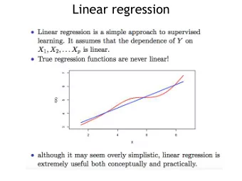
Regression Regression with one predictor y i = β 0 + β 1 x i + ǫ i Assumption: given x i , the response y i ∼ N ( β 0 + β 1 x i , σ 2 ), and y i are independent for all i . This extends directly to regression with multiple predictors y i = X i β + ǫ i with equivalent assumptions. Any statistics package will provide a best fit solution to these linear models, including standard errors for each β j and statistics describing the proportion of the total variance in y explained by the model. In R, we use lm() and in SAS we use PROC REG.

Regression diagnostics Regression diagnostics are about checking model assumptions and looking out for influential points. softbacks.lm <- lm( weight ~ volume, data = softbacks ) summary( softbacks.lm ) Coefficients: Estimate Std. Error t value Pr(>|t|) (Intercept) 41.3725 97.5588 0.424 0.686293 volume 0.6859 0.1059 6.475 0.000644 *** --- Signif. codes: 0 ’***’ 0.001 ’**’ 0.01 ’*’ 0.05 ’.’ 0.1 ’ ’ 1 Residual standard error: 102.2 on 6 degrees of freedom Multiple R-squared: 0.8748, Adjusted R-squared: 0.8539 F-statistic: 41.92 on 1 and 6 DF, p-value: 0.0006445

Regression diagnostics plot( softbacks.lm, which = 1:4 ) Residuals vs Fitted Normal Q−Q Standardized residuals 200 6 ● 6 ● 2 Residuals 100 1 ● ● ● 0 ● 0 ● ● ● ● ● ● −100 ● −1 1 ● 1 ● 4 ● 4 400 600 800 1000 −1.5 −0.5 0.5 1.5 Fitted values Theoretical Quantiles Scale−Location Cook's distance Standardized residuals 1.2 1.5 6 ● 4 Cook's distance 4 ● 1.0 0.8 ● 1 6 0.5 0.4 ● ● ● ● 1 ● 0.0 0.0 400 600 800 1000 1 2 3 4 5 6 7 8 Fitted values Obs. number

Intervals, tests, robust regression Once we have the model fit, we can obtain confidence intervals and do hypothesis testing on model parameters. We can also obtain prediction intervals for a future observation. In R, we can use predict( softbacks.lm , newdata = data.frame( volume = 1200 ) , interval = "prediction" ) fit lwr upr 864.4035 584.5337 1144.273 predict( softbacks.lm , newdata = data.frame( volume = 1200 ) , interval = "confidence" ) fit lwr upr 864.4035 738.7442 990.0628 In SAS, PROC REG has the same functionality in its OUTPUT statement.

Transformations We have seen several examples where a transformation improves contrast, linearity, and/or variance properties. The Box-Cox transformation is a generalized power transformation � y λ − 1 λ � = 0 λ y ( λ ) = log( y ) λ = 0 Box−Cox transformation for λ = −2, −1, −0.5, 0, 0.5, 1, 2 2 0 y ( λ ) −2 −4 0 1 2 3 4 y

Suggested steps for multiple regression ◮ Check the distributions of the dependent and explanatory variables (skewness, outliers) ◮ Plot a scatterplot matrix. Look for: ◮ Non-linearities ◮ Sufficient contrast ◮ (near) Collinearity ◮ Consider whether there are large errors in the explanatory variables (assumed known) ◮ Leads to errors in coefficient estimates ◮ Consider transformations to improve linearity and/or symmetry of distributions ◮ In the case of (near) collinearity, consider removing redundant explanatory variables ◮ After fitting the model, check residuals, Cook’s distances, and other diagnostics

Interpreting model coefficients ◮ When the goal is scientific understanding, we want to interpret model coefficients ◮ Data on brain weight, body weight, and litter size of 20 mice 6 7 8 9 12 ● ● ● ● ● ● ● ● 10 ● ● ● ● ● ● ● ● lsize ● ● ● ● 8 ● ● ● ● ● ● ● ● 6 ● ● ● ● ● ● ● ● 4 ● ● ● ● ● ● ● ● ● ● ● ● ● ● 9 ● ● ● ● ● ● ● ● 8 bodywt ● ● ● ● ● ● ● ● ● ● 7 ● ● ● ● ● ● ● ● ● ● 6 ● ● ● ● 0.44 ● ● ● ● ● ● ● ● ● ● ● ● ● ● ● ● 0.42 ● ● ● ● ● ● ● ● ● ● brainwt ● ● ● ● 0.40 ● ● ● ● ● ● 0.38 ● ● 4 6 8 10 12 0.38 0.40 0.42 0.44

> summary(lm( brainwt~ lsize, data = litters))$coef Estimate Std. Error t value Pr(>|t|) (Intercept) 0.44700 0.00962 46.44 3.39e-20 lsize -0.00403 0.00120 -3.37 3.44e-03 (No consideration of the effect of bodyweight on litter size. With this model, we might conclude that larger litter size is associated with smaller brain weight.) > summary(lm( brainwt~ lsize +bodywt, data = litters))$coef Estimate Std. Error t value Pr(>|t|) (Intercept) 0.17825 0.07532 2.37 0.03010 lsize 0.00669 0.00313 2.14 0.04751 bodywt 0.02431 0.00678 3.59 0.00228 (Coefficient for litter size measures change in brain weight when body weight is held constant. That is, for a particular body weight, larger litter size is associated with larger brain weight.)

Model selection criteria ◮ Model selection is the process of choosing a model among a set of candidate models ◮ Model selection is a combination of pre-defined procedure and statitstical judgment ◮ The model selection procedure should be based on the goal of the analysis (hypothesis testing? estimation? prediction?) ◮ Examples: ◮ Hypothesis testing on each coefficient (t-test) ◮ Total model comparison using hypothesis testing (F-test) ◮ Total model comparison using information criterion (AIC, BIC) ◮ Prediction performance on a test set ◮ Cross validation

Simulation experiment (in book) The authors did the following experiment: ◮ Generate 41 vectors of 100 independent random normally-distributed numbers ◮ Label the first vector as y , the response, and the remaining as X , the explanatory variables ◮ Look for the three x variables that best explain y . How many are statistically significant? Cases All three variables were significant at p < 0.01 1 All three variables significant at p < 0.05 3 Two of three significant at p < 0.05 3 One significant at p < 0.05 3 Total 10 ◮ p-values do not account for variable selection and structural uncertainties!

Assessing predictive power ◮ In some cases, we use regression to obtain a model that can be used for prediction ◮ How do we decide on a model for prediction? ◮ We are looking for a model that will minimize L (ˆ y ( θ, X future ) , y ( X future )) ◮ If we have the true model, then ˆ y () is the same as y () (trivial) ◮ Do we have the true model? What kinds of errors can we make? ◮ Finite sample errors (don’t observe enough data to pin down θ ) ◮ Structural errors (wrong class of model, wrong covariates) ◮ Are we using the appropriate criterion? ◮ Hypothesis testing is likely not the correct choice here ◮ Prediction error is better

Cross-validation How can we get a handle on prediction error? ◮ Divide our sample into a training set and a test set ◮ Use our training set to obtain a set of prediction models ◮ Predict the test set using the prediction models and compare Cross-validation is an extension of this idea ◮ Divide the data into k sets (folds) ◮ Leave one fold out, obtain model ◮ Repeat for each fold ◮ Average over the k sets of results You can use cross-validation to do variable selection, but you need to use another set of data to estimate coefficients, standard errors, etc.

Multicollinearity ◮ Explanatory variables that are (nearly) linear combinations of other explanatory variables are collinear . ◮ Extreme example is compositional data (fractions of a whole). ◮ Example from book: 25 specimens of rock ◮ Percentage by weight of five minerals (albite, blandite, cornite, daubite, endite) ◮ Depth at which sample collected ◮ Porosity ◮ Note that the composition data has to add to 100% (if we know four of five, we can calculate the fifth)