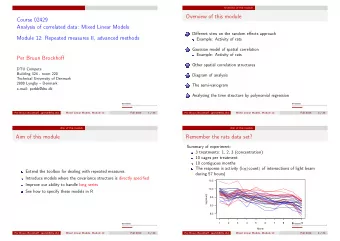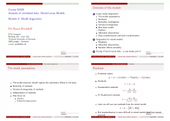
Oversigt Course 02429 Analysis of correlated data: Mixed Linear - PowerPoint PPT Presentation
Overview Oversigt Course 02429 Analysis of correlated data: Mixed Linear Models Module 1: Introduction to mixed models Overview 1 Simple intro example 2 Per Bruun Brockhoff The mixed model 3 DTU Compute Building 324 - room 220 Missing
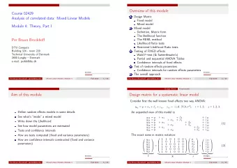
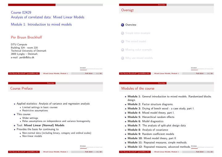
Overview Oversigt Course 02429 Analysis of correlated data: Mixed Linear Models Module 1: Introduction to mixed models Overview 1 Simple intro example 2 Per Bruun Brockhoff The mixed model 3 DTU Compute Building 324 - room 220 Missing value example 4 Technical University of Denmark 2800 Lyngby – Denmark e-mail: perbb@dtu.dk Why use mixed models 5 Per Bruun Brockhoff (perbb@dtu.dk) Mixed Linear Models, Module 1 Fall 2014 1 / 20 Per Bruun Brockhoff (perbb@dtu.dk) Mixed Linear Models, Module 1 Fall 2014 2 / 20 Overview Overview Course Preface Modules of the course Module 1: General introduction to mixed models. Randomized blocks design. Applied statistics: Analysis of variance and regression analysis Module 2: Factor structure diagrams. Limited settings in basic courses Module 3: Drying of beech wood - a case study, part I. Restrictive assumptions Module 4: Mixed model theory, part I. This course: Module 5: Hierarchical random effects Wider settings Relax assumptions on independence and variance homogeneity Module 6: Model diagnostics Tool: Mixed Linear (Normal) Models Module 7: The analysis of split-plot design data Provides the basis for continuing to Module 8: Analysis of covariance Non-normal data (including binary, category and ordinal scales) Module 9: Random coefficient models Non-linear models Module 10: Mixed model theory, part II Module 11: Repeated measures, simple methods. Module 12: Repeated measures, advanced methods. Per Bruun Brockhoff (perbb@dtu.dk) Mixed Linear Models, Module 1 Fall 2014 3 / 20 Per Bruun Brockhoff (perbb@dtu.dk) Mixed Linear Models, Module 1 Fall 2014 4 / 20
Overview Simple intro example Content of Module 1: Oversigt Overview 1 Course material preface Introductory example. Simple intro example 2 Randomized blocks design. Random versus fixed block effect. The mixed model 3 Comparison of fixed and mixed model. Example with missing values. Missing value example 4 Why use mixed models? R introduction. Why use mixed models 5 Per Bruun Brockhoff (perbb@dtu.dk) Mixed Linear Models, Module 1 Fall 2014 5 / 20 Per Bruun Brockhoff (perbb@dtu.dk) Mixed Linear Models, Module 1 Fall 2014 6 / 20 Simple intro example Simple intro example Introductory example: NIR predictions of HPLC Simple analysis by paired t-test measurements The uncertainty of the estimated difference: SE d = s d √ n = 0 . 2953 √ = 0 . 0934 Data: 10 HPLC NIR Difference Hypothesis test: Tablet 1 10.4 10.1 0.3 d = − 0 . 05 Tablet 2 10.6 10.8 -0.2 t = 0 . 0934 = − 0 . 535 SE d Tablet 3 10.2 10.2 0.0 Tablet 4 10.1 9.9 0.2 A 95%-confidence band: Tablet 5 10.3 11 -0.7 d ± t 0 . 975 (9) SE d ⇐ ⇒ − 0 . 05 ± 0 . 21 Tablet 6 10.7 10.5 0.2 Tablet 7 10.3 10.2 0.1 Result: No significant method difference. (P-value = 0 . 61 ) Tablet 8 10.9 10.9 0.0 The statistical model: Tablet 9 10.1 10.4 -0.3 d i = µ + ε i , ε ∼ N (0 , σ 2 ) , Tablet 10 9.8 9.9 -0.1 Aim: Study the method differences. Model parameter estimates: µ = d, ˆ σ = s d ˆ Per Bruun Brockhoff (perbb@dtu.dk) Mixed Linear Models, Module 1 Fall 2014 7 / 20 Per Bruun Brockhoff (perbb@dtu.dk) Mixed Linear Models, Module 1 Fall 2014 8 / 20
Simple intro example Simple intro example Simple analysis by an ANOVA approach The problem of the ANOVA approach The uncertainty of the average NIR value within the model: Randomized Blocks setup with 10 "blocks" (the tablets) and two "treatments" (the methods): ˆ σ SE ( y 1 ) = √ 10 = 0 . 066 y ij = µ + α i + β j + ε ij , ε ij ∼ N (0 , σ 2 ) , This is "wrong"! Same analysis as the paired t-test: The tablet-to-tablet variation is ignored. Source of Degrees of Sums of Mean F P Using ONLY the 10 NIR-values gives: variation freedom squares squares s 1 s 1 = 0 . 4012 , SE ( y 1 ) = √ 10 = 0 . 127 Tablets 9 2.0005 0.2223 5.10 0.0118 Methods 1 0.0125 0.0125 0.29 0.6054 The ANOVA approach: Residual 9 0.3925 0.0436 Is valid only for statements about the 10 specific tablets in the The uncertainty of the average method difference: experiment. The 2nd approach: � 1 � 10 + 1 � Considers the 10 tablets as a random sample. (But ignores the SE ( y 2 − y 1 ) = σ 2 ˆ = 0 . 0934 information from the HPLC measurements) 10 Is valid for tablets in general. Per Bruun Brockhoff (perbb@dtu.dk) Mixed Linear Models, Module 1 Fall 2014 9 / 20 Per Bruun Brockhoff (perbb@dtu.dk) Mixed Linear Models, Module 1 Fall 2014 10 / 20 The mixed model The mixed model Oversigt The solution: Overview 1 Combine the random sample assumption with a model for the entire data set! Simple intro example 2 The mixed linear model: Considers the tablet differences as random effects : The mixed model 3 y ij = µ + a i + β j + ε ij , ε ij ∼ N (0 , σ 2 ) , a i ∼ N (0 , σ 2 T ) . Missing value example 4 Note: Statements about method DIFFERENCES are the same for the two kinds of validity. Why use mixed models 5 Per Bruun Brockhoff (perbb@dtu.dk) Mixed Linear Models, Module 1 Fall 2014 11 / 20 Per Bruun Brockhoff (perbb@dtu.dk) Mixed Linear Models, Module 1 Fall 2014 12 / 20
The mixed model The mixed model Comparison of fixed and mixed model Analysis by mixed model ANOVA table as for the fixed model: A model can be characterized by three features: Source of Degrees of Sums of Mean E(MS) The expected value of the ij th observation y ij 1 variation freedom squares squares The variance of the ij th observation y ij 2 2 σ 2 T + σ 2 The relation between two different observations Tablets 9 2.0005 0.2223 3 σ 2 + 10 � β 2 (covariance/correlation) Methods 1 0.0125 0.0125 j σ 2 Residual 9 0.3925 0.0436 A comparison of the two models: Variance components estimated by: Fixed model Mixed model 1. E ( y ij ) µ + α i + β j µ + β j T = 0 . 2223 − 0 . 0436 σ 2 = 0 . 0436 , ˆ σ 2 σ 2 T + σ 2 σ 2 2. var ( y ij ) ˆ = 0 . 0894 2 ′ ) σ 2 3. cov ( y ij , y i ′ j ′ ) 0 T (if i = i ′ ) ′ ) The uncertainty of the average NIR-value in the mixed model is: ( j � = j 0 (if i � = i In summary: (for the mixed model) � √ 0 . 0894 + 0 . 0436 σ 2 σ 2 ˆ T + ˆ The tablet differences become a part of the variance structure. SE ( y 1 ) = √ = √ = 0 . 115 The observations are no longer independent 10 10 Per Bruun Brockhoff (perbb@dtu.dk) Mixed Linear Models, Module 1 Fall 2014 13 / 20 Per Bruun Brockhoff (perbb@dtu.dk) Mixed Linear Models, Module 1 Fall 2014 14 / 20 Missing value example Missing value example Oversigt Example with missing values Data: HPLC NIR Difference Tablet 1 10.4 10.1 0.3 Overview 1 Tablet 2 10.6 10.8 -0.2 Tablet 3 10.2 10.2 0.0 Tablet 4 10.1 9.9 0.2 Tablet 5 10.3 11 -0.7 Simple intro example 2 Tablet 6 10.7 10.5 0.2 Tablet 7 10.3 10.2 0.1 Tablet 8 10.9 10.9 0.0 The mixed model 3 Tablet 9 10.1 10.4 -0.3 Tablet 10 9.8 9.9 -0.1 Tablet 11 10.8 Tablet 12 9.8 Missing value example 4 Tablet 13 10.5 Tablet 14 10.3 Tablet 15 9.7 Why use mixed models 5 Tablet 16 10.3 Tablet 17 9.6 Tablet 18 10.0 Tablet 19 10.2 Tablet 20 9.9 Per Bruun Brockhoff (perbb@dtu.dk) Mixed Linear Models, Module 1 Fall 2014 15 / 20 Per Bruun Brockhoff (perbb@dtu.dk) Mixed Linear Models, Module 1 Fall 2014 16 / 20
Missing value example Missing value example Analysis by fixed effects ANOVA Analysis by mixed model The results (as given by PROC MIXED in SAS): σ 2 = 0 . 0435 , ANOVA table: σ 2 ˆ ˆ T = 0 . 1019 Source of Degrees of Sums of Mean F P β 2 − ˆ ˆ SE (ˆ β 2 − ˆ β 1 = − 0 . 07211 , β 1 ) = 0 . 0870 variation freedom squares squares Tablets 19 3.7230 0.1959 4.49 0.0129 Information from all data is used! Methods 1 0.0125 0.0125 0.29 0.6054 Consider ONLY tablets 11-20: Two (independent) samples t-test setup Residual 9 0.3925 0.0436 with 5 tablets in each group: The results for the method differences EXACTLY as before: y 1 = 10 . 22 , s 1 = 0 . 4658 , y 2 = 10 . 00 , s 2 = 0 . 2739 � 1 � 10 + 1 � SE (ˆ β 2 − ˆ σ 2 β 1 ) = ˆ = 0 . 0934 The results from the two separate analyzes can be summarized as: 10 Tablets 1-10 Tablets 11-20 Difference -0.05 -0.22 The information in Tablets 11-20 are NOT used! SE 2 0.00872 0.0584 The mixed model analysis combines these two sets of information! Per Bruun Brockhoff (perbb@dtu.dk) Mixed Linear Models, Module 1 Fall 2014 17 / 20 Per Bruun Brockhoff (perbb@dtu.dk) Mixed Linear Models, Module 1 Fall 2014 18 / 20 Why use mixed models Why use mixed models Oversigt Why use mixed models? Overview 1 To avoid mistakes. Simple intro example 2 To broaden the statistical inference. To recover all relevant information in the data. The mixed model 3 To be able to handle correlation structures in the data. To be able to handle non-homogeneous variances. Missing value example 4 To use the only reasonable model for the data! Why use mixed models 5 Per Bruun Brockhoff (perbb@dtu.dk) Mixed Linear Models, Module 1 Fall 2014 19 / 20 Per Bruun Brockhoff (perbb@dtu.dk) Mixed Linear Models, Module 1 Fall 2014 20 / 20
Recommend
More recommend
Explore More Topics
Stay informed with curated content and fresh updates.
