Oversigt Course 02429 Analysis of correlated data: Mixed Linear - PowerPoint PPT Presentation

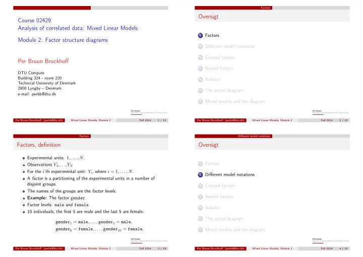
Factors Oversigt Course 02429 Analysis of correlated data: Mixed Linear Models Factors 1 Module 2: Factor structure diagrams Different model notations 2 Crossed factors 3 Per Bruun Brockhoff Nested factors 4 DTU Compute Building 324 - room 220 Balance 5 Technical University of Denmark 2800 Lyngby – Denmark The actual diagram 6 e-mail: perbb@dtu.dk Mixed models and the diagram 7 Per Bruun Brockhoff (perbb@dtu.dk) Mixed Linear Models, Module 2 Fall 2014 1 / 19 Per Bruun Brockhoff (perbb@dtu.dk) Mixed Linear Models, Module 2 Fall 2014 2 / 19 Factors Different model notations Factors, definition Oversigt Experimental units: 1 , . . . , N . Factors 1 Observations Y 1 ,. . . , Y N For the i ’th experimental unit: Y i , where i = 1 , . . . , N . Different model notations 2 A factor is a partitioning of the experimental units in a number of disjoint groups. Crossed factors 3 The names of the groups are the factor levels . Nested factors 4 Example: The factor gender . Factor levels: male and female . Balance 5 10 individuals, the first 5 are male and the last 5 are female: The actual diagram 6 gender 1 = male , . . . , gender 5 = male , gender 6 = female , . . . , gender 10 = female . Mixed models and the diagram 7 Per Bruun Brockhoff (perbb@dtu.dk) Mixed Linear Models, Module 2 Fall 2014 3 / 19 Per Bruun Brockhoff (perbb@dtu.dk) Mixed Linear Models, Module 2 Fall 2014 4 / 19

Different model notations Crossed factors Model notations Oversigt The "usual" model expression: (for the "gender example") Factors 1 Y ij = µ + α i + ǫ ij , j = 1 , . . . , 5 , i = 1 , 2 Different model notations 2 A more general (and better) model expression: Crossed factors 3 Y i = µ ( gender i ) + ǫ i Nested factors 4 with the two mean value structure (fixed) parameters µ ( male ) and µ ( female ) . Balance 5 Or equivalently: The actual diagram Y i = µ + α ( gender i ) + ǫ i 6 With "quantitative elements" in a model, e.g. a classical regression Mixed models and the diagram 7 model: Y i = α + β · x i + ǫ i Per Bruun Brockhoff (perbb@dtu.dk) Mixed Linear Models, Module 2 Fall 2014 5 / 19 Per Bruun Brockhoff (perbb@dtu.dk) Mixed Linear Models, Module 2 Fall 2014 6 / 19 Crossed factors Crossed factors Crossed factors Crossed factors, cont. Two factors: Let F and G be two factors in an experiment. atm with 2 levels: norm and mod The product factor , F × G : temp with 3 levels: 5, 10, 15. The product factor atm × temp has six levels: ( F × G ) i = ( F i , G i ) ( norm , 5) , ( norm , 10) , ( norm , 15) , Used for interactions. ( mod , 5) , ( mod , 10) , ( mod , 15) . Example: 6 vegetables were stored under different conditions. Each combination of: Model expression (2-way ANOVA): Two atmosphere conditions: normal or modified. Three temperature conditions: 5, 10 or 15 centigrades (celcius). E Y = α ( atm ) + β ( temp ) + γ ( atm × temp ) . Per Bruun Brockhoff (perbb@dtu.dk) Mixed Linear Models, Module 2 Fall 2014 7 / 19 Per Bruun Brockhoff (perbb@dtu.dk) Mixed Linear Models, Module 2 Fall 2014 8 / 19

Nested factors Nested factors Oversigt Nested factors F finer than G if the partitioning according to F ’s levels is a sub-partitioning of the groups obtained by the partitioning according Factors 1 to G ’s levels. Different model notations Nested structure = hierarchical structure 2 Example: 3 Repeated observations on 8 piglets from 2 different Crossed factors 3 litters: Litter=1 Litter=2 Nested factors 4 Pig=1 Pig=2 Pig=3 Pig=4 Pig=5 Pig=6 Pig=7 Pig=8 Balance 5 1 2 3 4 5 6 7 8 9 10 11 12 13 14 15 16 17 18 19 20 21 22 23 24 The factor piglet is finer than the factor litter . The actual diagram 6 The factor piglet is nested within the factor litter . The factor litter is coarser than the factor piglet . Mixed models and the diagram 7 The litter effect is contained in the piglet effect. A product factor is always finer than each of the individual factors. Per Bruun Brockhoff (perbb@dtu.dk) Mixed Linear Models, Module 2 Fall 2014 9 / 19 Per Bruun Brockhoff (perbb@dtu.dk) Mixed Linear Models, Module 2 Fall 2014 10 / 19 Balance Balance Oversigt Balance Factors 1 A factor is balanced , if there are the same number of experimental units for each level of the factor. Different model notations 2 If atm × temp is balanced, then atm and temp will be balanced. Crossed factors Balance of single factors can occur under less restrictive assumptions. 3 Some possible pleasant consequences of (a certain degree of) balance Nested factors are that: 4 ANOVA tables are unique. Balance 5 Estimates of fixed effects levels equal their raw means. Estimates of fixed effect levels do not change even though random The actual diagram effects are considered fixed. 6 In many cases, tests for the significance of fixed and/or random effects in the mixed model become simple F-tests. Mixed models and the diagram 7 Per Bruun Brockhoff (perbb@dtu.dk) Mixed Linear Models, Module 2 Fall 2014 11 / 19 Per Bruun Brockhoff (perbb@dtu.dk) Mixed Linear Models, Module 2 Fall 2014 12 / 19

The actual diagram The actual diagram Oversigt The factor structure diagrams Storage example: 5 vegetables in each of the 6 conditions Factors 1 30 experimental units Factors: Different model notations 2 atm , temp , atm × temp . Crossed factors 3 Basic factors always present: The constant factor called 0 , where the factor level is 0 for all Nested factors 4 experimental units. The unit factor I that partitions each experimental unit into its own Balance 5 group consisting of only this one experimental unit. Factors: The actual diagram 6 0 , atm , temp , atm × temp , I . Corresponding to the model expression: Mixed models and the diagram 7 Y i = µ + α ( atm i ) + β ( temp i ) + γ ( atm × temp i ) + ǫ i , i = 1 , . . . , 30 , Per Bruun Brockhoff (perbb@dtu.dk) Mixed Linear Models, Module 2 Fall 2014 13 / 19 Per Bruun Brockhoff (perbb@dtu.dk) Mixed Linear Models, Module 2 Fall 2014 14 / 19 The actual diagram The actual diagram The factor structure diagrams The factor structure diagrams in R library(diagram) ## Creating the list of factor names with indices: names=c(expression("[I]"[24]^{30}),expression(atm:temp[2]^{6}), expression(atm[1]^{2}), expression(temp[2]^{3}),expression(0[1]^{1})) 2 atm 1 ## Since there are 5 factors create the 5x5 matrix of zeros: atm × temp 2 30 6 1 [I] 24 0 1 M <- matrix(nrow = 5, ncol = 5, byrow = TRUE, data = 0) ## Envision the structure: e.g. I need an arrow from my first ## name to my second name so assign something to M[2,1] etc: 3 temp 2 M[2, 1] <- M[3,2] <- M[4, 2] <- M[5,3] <- M[5,4] <- "." ## Make the diagram: plotmat(M, pos = c(1, 1, 2, 1), name = names, lwd = 2, box.lwd = 1, cex.txt = 1, box.size = 0.1, Shows all factors (model terms) box.type = "square", box.prop = 0.5, arr.type="triangle",curve=0) Structure: Arrows from finer to coarser factors. Degrees of freedom: Lower indices – can be calculated easily. Per Bruun Brockhoff (perbb@dtu.dk) Mixed Linear Models, Module 2 Fall 2014 15 / 19 Per Bruun Brockhoff (perbb@dtu.dk) Mixed Linear Models, Module 2 Fall 2014 16 / 19

The actual diagram Mixed models and the diagram The factor structure diagrams in R Oversigt 30 [I] 24 Factors 1 . atm : temp 2 6 Different model notations 2 . . Crossed factors 3 2 3 atm 1 temp 2 Nested factors 4 . . 1 0 1 Balance 5 The actual diagram 6 Mixed models and the diagram 7 Per Bruun Brockhoff (perbb@dtu.dk) Mixed Linear Models, Module 2 Fall 2014 17 / 19 Per Bruun Brockhoff (perbb@dtu.dk) Mixed Linear Models, Module 2 Fall 2014 18 / 19 Mixed models and the diagram Random effects in diagrams Illustrated by use of brackets . The unit(residual) factor is always random: [I]. The diagram tells us how to test the fixed effects in a mixed model (in "nice" cases): Error stratum : A Random effect "pointing at" a fixed effect should be used as the error term for inference about this fixed effect. Per Bruun Brockhoff (perbb@dtu.dk) Mixed Linear Models, Module 2 Fall 2014 19 / 19