Markov Decision Processes II School of Data Science, Fudan - PowerPoint PPT Presentation

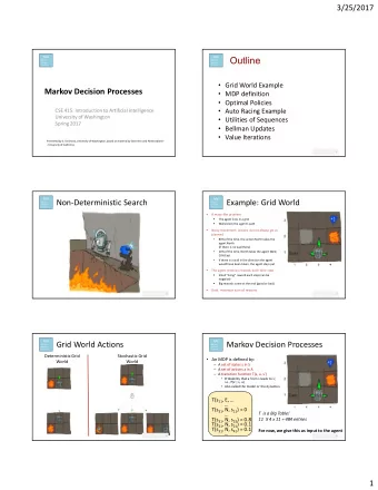
DATA130008 Introduction to Artificial Intelligence Markov Decision Processes II 魏忠钰 复旦大学大数据学院 School of Data Science, Fudan University April 10 th , 2019

Policy Extraction

� Computing Actions from Values § Let’s imagine we have the optimal values V*(s) § How should we act? § We need to do an expectimax (one step) 𝜌 ∗ 𝑡 = argmax 0 𝑄 𝑡 2 𝑡, 𝑏 𝑊 ∗ (𝑡 2 ) *∈,(.) . 7 This is called policy extraction, since it gets the policy implied by the values

Computing Actions from Q-Values § Let’s imagine we have the optimal q-values: § How should we act? Important lesson: actions are easier to select from q- values than values!

� Problems with Value Iteration § Value iteration repeats the Bellman updates: *∈,(.) 0 𝑄 𝑡 2 𝑡, 𝑏 𝑊 8 (𝑡 2 ) 𝑊 89: 𝑡 ← 𝑆 𝑡 + 𝛿 max s . 7 a s, a s,a,s ’ s ’ § Problem 1: It’s slow – O(S 2 A) per iteration § Problem 2: The “max” at each state rarely changes § Problem 3: The policy often converges long before the values

Policy Methods

Policy Evaluation

Fixed Policies Do the optimal action Do what p says to do s s p (s) a s, p (s) s, a s,a,s ’ s, p (s),s ’ s ’ s ’ § Expectimax trees max over all actions to compute the optimal values § If we fixed some policy p (s), then the tree would be simpler – only one action per state § … though the tree’s value would depend on which policy we fixed

� Utilities for a Fixed Policy § Another basic operation: compute the utility of a state s under a fixed (generally non-optimal) policy § Define the utility of a state s, under a fixed policy p : § V p (s) = expected total discounted rewards starting in s and following p § Recursive relation (one-step look-ahead / Bellman equation): s 0 𝑄 𝑡 2 𝑡, 𝑏 V p (𝑡 2 ) V p (s) ← 𝑆 𝑡 + 𝛿 . 7 p (s) s, p (s) s, p (s),s ’ s ’

Example: Policy Evaluation Always Go Right Always Go Forward

Example: Policy Evaluation Always Go Forward Always Go Right

Bellman Equation (policy) in Matrix Form § The Bellman equation can be expressed concisely using matrices 𝑤 = R + γ𝑄𝑤 § Where v is a column vector with one entry per state

Solving the Bellman Equation (policy) § The Bellman equation (policy) is a linear equation § It can be solved directly § Computational complexity is O(n 3 ) for n states § Direct solution only possible for small MDPs

� Solving the Bellman Equation (policy) § Iteration: Turn recursive Bellman equations into updates s (like value iteration) p (s) s, p (s) A (𝑡) ← 𝑆 𝑡 + 𝛿 0 𝑄 𝑡 2 𝑡, 𝑏 𝑊 A (𝑡 2 )) 𝑊 89: 8 . 7 s, p (s),s ’ § Efficiency: O(S 2 ) per iteration s ’

Policy Iteration

Policy Iteration § Alternative approach for optimal values: § Step 1: Policy evaluation: calculate utilities for some fixed policy (not optimal utilities!) until convergence § Step 2: Policy improvement: update policy using one-step look-ahead with resulting converged (but not optimal!) utilities as future values § Repeat steps until policy converges § This is policy iteration § It’s still optimal! § Can converge (much) faster under some conditions

Policy Iteration § Evaluation: For fixed current policy p , find values with policy evaluation: U i = U π i § Iterate until values converge: § Improvement: For fixed values, get a better policy using policy extraction § One-step look-ahead:

Policy Iteration

Policy Iteration

Modified Policy Iteration § Does policy evaluation need to converge to 𝑤 A ? § Or should we introduce a stopping condition § E.g. epsilon-convergence of value function § Or simply stop after k iterations of iterative policy evaluation? § Why not update policy every iteration? i.e. stop after k = 1 § This is equivalent to value iteration.

Comparison § Both value iteration and policy iteration compute the same thing (all optimal values) § In value iteration: § Every iteration updates both the values and (implicitly) the policy § We don’t track the policy, but taking the max over actions implicitly re-computes it § In policy iteration: § We do several passes that update utilities with fixed policy (each pass is fast because we consider only one action, not all of them) § After the policy is evaluated, a new policy is chosen (slow like a value iteration pass) § The new policy will be better § Both are dynamic programs for solving MDPs

Summary: MDP Algorithms § So you want to…. § Compute optimal values: use value iteration or policy iteration § Compute values for a particular policy: use policy evaluation § Turn your values into a policy: use policy extraction (one-step lookahead) § These all look the same! § They are all variations of Bellman updates § They all use one-step look-ahead expectimax fragments § They differ only in whether we plug in a fixed policy or max over actions

Synchronous Dynamic Programming Algorithms § Both value iteration and policy iteration used synchronous backups § i.e. all states are backup up in parallel § Asynchronous DP backs up states individually, in any order § For each selected state, apply the appropriate backup § Can significantly reduce computation § Guaranteed to converge if all states continue to be selected

Synchronous Dynamic Programming Algorithms § Three simple ideas for asynchronous dynamic programming: § In-place dynamic programming § Prioritiesd sweeping § Real-time dynamic programming

In-place Dynamic Programming § Synchronous value iteration stores two copies of value function § For all s in S § In-place value iteration only stores one copy of value function § For all s in S

Prioritised Sweeping § Use magnitude of Bellman error to guide state selection, e.g. § Backup the state with the largest remaining Bellman error § Update Bellman error of affected states after each backup § Can be implemented efficiently by maintaining a priority queue

Real-Time Dynamic Programming § Idea: only states that are relevant to agent § Use agent’s experience to guide the selection of states § After each time-step § Backup the state 𝑇 C § § Focus the DP’s backups onto parts of states that are most relevant to the agents

Full-Width Backups § DP uses full-width backups § For each backup (sync or async) § Every successor state and action is considered § Using knowledge of the MDP transitions and reward function § DP is effective for medium-sized problems (millions of states) § For large problems DP suffers Bellman’s curse of dimensionality § Number of states n = |S| grows exponentially with number of state variables s § Each one backup can be too expensive then a s, a s,a,s s ’ ’

Sample Backups § Using sample rewards and sample transitions instead of reward function R and transition dynamics P § Advantages: § Model free: no advance knowledge of MDP required § Breaks the curse of dimensionality through sampling § Cost of backup is constant, independent of n = |S|

Double Bandits

Double-Bandit MDP § Actions: Blue, Red § States: Win, Lose No discount 100 time steps Both states have the same value 0.25 $0 0.75 $2 0.25 W L $0 $1 $1 0.75 $2 1.0 1.0

Offline Planning § Solving MDPs is offline planning § You determine all quantities through computation § You need to know the details of the MDP No discount § You do not actually play the game! 100 time steps Both states have the same value Value 0.25 $0 Play Red 150 0.75 0.25 W L $2 $0 $1 $1 Play Blue 100 0.75 $2 1.0 1.0

Let's Play! $2 $2 $0 $2 $2 $2 $2 $0 $0 $0

Online Planning § Rules changed! Red’s win chance is different. ?? $0 ?? $2 W ?? L $0 $1 $1 ?? $2 1.0 1.0

Let's Play! $0 $0 $0 $2 $0 $2 $0 $0 $0 $0

What Just Happened? § That wasn’t planning, it was learning! § Specifically, reinforcement learning § There was an MDP, but you couldn’t solve it with just computation § You needed to actually act to figure it out § Important ideas in reinforcement learning that came up § Exploration: you have to try unknown actions to get information § Exploitation: eventually, you have to use what you know § Regret: even if you learn intelligently, you make mistakes § Sampling: because of chance, you have to try things repeatedly § Difficulty: learning can be much harder than solving a known MDP